Validating Modern Machine Learning (ML) Methods Prior to Productionization

Last time, we discussed the steps that a modeler must pay attention to when building out ML models to be utilized within the financial institution. In summary, to ensure that they have built a robust model, modelers must make certain that they have designed the model in a way that is backed by research and industry-adopted practices. DataRobot assists the modeler in this process by providing tools that are aimed at accelerating and automating critical steps of the model development process—from flagging potential data quality issues to trying out multiple model architectures, these tools not only conform to the expectations laid out by SR 11-7, but also give the modeler a wider tool kit in adopting sophisticated algorithms in the enterprise setting.

In this post, we will dive deeper into how members from both the first and second line of defense within a financial institution can adapt their model validation strategies in the context of modern ML methods. Further, we will discuss how DataRobot is able to help streamline this process, by providing various diagnostic tools aimed at thoroughly evaluating a model’s performance prior to placing it into production.

Validating Machine Learning Models 

If we have already built out a model for a business application, how do we ensure that it is working to our expectations? What are some steps that the modeler/validator must take to evaluate the model and ensure that it is a strong fit for its design objectives?

To start with, SR 11-7 lays out the criticality of model validation in an effective model risk management practice: 

Model validation is the set of processes and activities intended to verify that models are performing as expected, in line with their design objectives and business uses. Effective validation helps ensure that models are sound. It also identifies potential limitations and assumptions, and assesses their possible impact.

SR 11-7 further goes to detail the components of an effective validation, which includes: 

1. Evaluation of conceptual soundness
2. Ongoing monitoring
3. Outcomes analysis

While SR 11-7 is prescriptive in its guidance, one challenge that validators face today is adapting the guidelines to modern ML methods that have proliferated in the past few years. When the FRB’s guidance was first introduced in 2011, modelers often employed traditional regression-based models for their business needs. These methods provided the benefit of being supported by rich literature on the relevant statistical tests to confirm the model’s validity—if a validator wanted to confirm that the input predictors of a regression model were indeed relevant to the response, they need only to construct a hypothesis test to validate the input. Furthermore, due to their relative simplicity in model structure, these models were very straightforward to interpret. However, with the widespread adoption of modern ML techniques, including gradient-boosted decision trees (GBDTs) and deep learning algorithms, many traditional validation techniques become difficult or impossible to apply. These newer approaches often have the benefit of higher performance compared to regression-based approaches, but come at the cost of added model complexity. To deploy these models into production with confidence, modelers and validators need to adopt new techniques to ensure the validity of the model. 

Conceptual Soundness of the Model

Evaluating ML models for their conceptual soundness requires the validator to assess the quality of the model design and ensure it is fit for its business objective. Not only does this include reviewing the assumptions in selecting the input features and data, it also requires analyzing the model’s behavior over a variety of input values. This may be accomplished through a wide variety of tests, to develop a deeper introspection into how the model behaves.

Model explainability is a critical component of understanding a model’s behavior over a spectrum of input values. Traditional statistical models like linear and logistic regression made this process relatively straightforward, as the modeler was able to leverage their domain expertise and directly encode factors relevant to the target they were trying to predict. In the model-fitting procedure, the modeler is then able to measure the impact of each factor against the outcome. In contrast, many modern ML methods may combine data inputs in non-linear ways to produce outputs, making model explainability more difficult, yet necessary prior to productionization. In this context, how does the validator ensure that the data inputs and model behavior matches their expectations? 

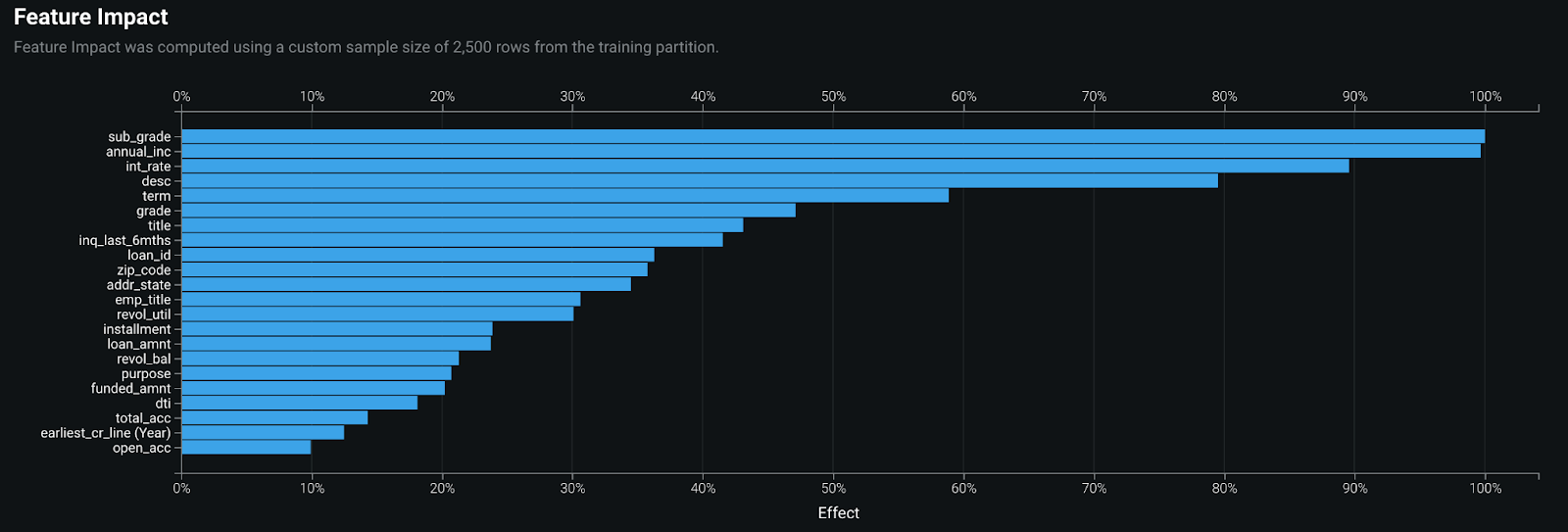
One approach is to assess the importance of the input variables in the model, and evaluate its impact on the outcome being predicted. Examining these global feature importances enables the validator to understand the top data inputs and ensure that they fit with their domain expertise. Within DataRobot, each model created in the model leaderboard contains a feature impact visualization, which makes use of a mathematical technique called permutation importance to measure variable importance. Permutation importance is model agnostic, making it perfect for modern ML approaches, and it works by measuring the impact of shuffling the values of an input variable against the performance of the model. The more important a variable is, the more negatively the model performance will be impacted by randomizing its values. 

As a concrete example, a modeler may be tasked with constructing a probability of default (PD) model. After building the model, the validator in the second line of defense may inspect the feature impact plot shown in Figure 1 below, to examine the most influential variables the model leveraged. As per the output, the two most influential variables were the grade of the loan assigned and the annual income of the applicant. Given the context of the problem, the validator may approve the model construction, as these inputs are context-appropriate. 

In addition to examining feature importances, another step a validator may take to review the conceptual soundness of a model is to perform a sensitivity analysis. To directly quote SR 11-7: 

Where appropriate to the model, banks should employ sensitivity analysis in model development and validation to check the impact of small changes in input and parameter values on model outputs to make sure they fall within an expected range.

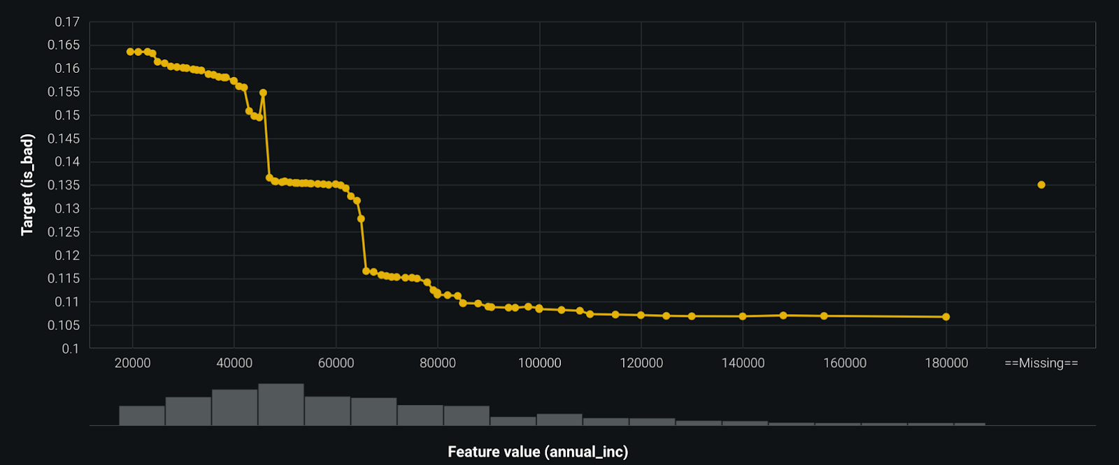
By examining the relationship the model learns between its inputs and outputs, the validator is able to confirm that the model is fit for its design objectives and that the model will yield reasonable outputs across a range of input values. Within DataRobot, the validator may look at the feature effects plot as shown in Figure 2 below, which makes use of a technique called partial dependence to highlight how the outcome of the model changes as a function of the input variable. Drawing from the probability of default model discussed earlier, we can see in the figure that the likelihood of an applicant defaulting on a loan decreases with an increase in their salary. This should make intuitive sense, as individuals with more financial reserves would pose the institution with a lower credit risk compared to those with less. 

Lastly, in contrast with the above approaches, a validator may make use of ‘local’ feature explanations to understand the additive contributions of each input variable against the model output. Within DataRobot, the validator may accomplish this by configuring the modeling project to make use of SHAP to produce these prediction explanations. This methodology assists in evaluating the conceptual soundness of a model by ensuring that the model adheres to domain-specific rules when making predictions, especially for modern ML approaches. Furthermore, it can foster trust between model consumers, as they are able to understand the factors driving a particular model outcome. 

Outcomes Analysis 

Outcomes Analysis is a core component of the model validation process, whereby the model’s outputs are compared against actual outcomes observed. These comparisons enable the modeler and validator alike to evaluate the model’s performance, and assess it against the business objectives for which it was created. In the context of machine learning models, many different statistical tests and metrics may be used to quantify the performance of a model, but as quoted by SR 11-7, is wholly dependent upon the model’s technique and intended use: 

The precise nature of the comparison depends on the objectives of a model, and might include an assessment of the accuracy of estimates or forecasts, an evaluation of rank-ordering ability, or other appropriate tests.

Out of the box, DataRobot provides a variety of different model performance metrics based on the model architecture used, and further empowers the modeler to do their own analysis by making available all model-related data through its API. For example, in the context of a supervised binary classification problem, DataRobot automatically calculates the model’s F1, Precision, and Recall score—performance metrics that capture the model’s ability to accurately identify classes of interest. Furthermore, through its interactive interface, the modeler is able to do multiple what-if analyses to see the impact of changing the prediction threshold on the corresponding model precision and recall. In the context of financial services, these metrics would be especially useful in evaluating the institution’s Anti-Money-Laundering (AML) models, where the model performance can be measured by the number of false positives it generates.

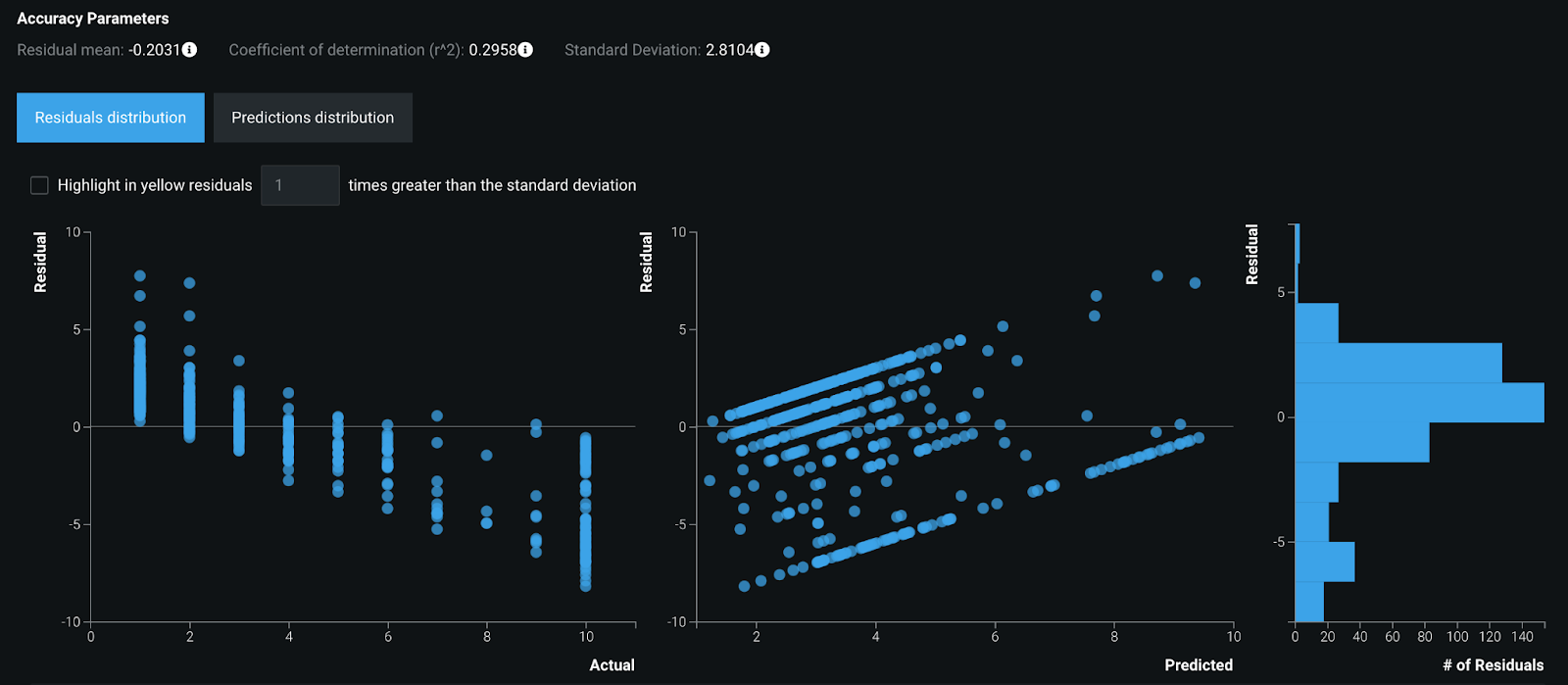
In addition to the model metrics discussed above for classification, DataRobot similarly provides fit metrics for regression models, and helps the modeler visualize the spread of model errors. 

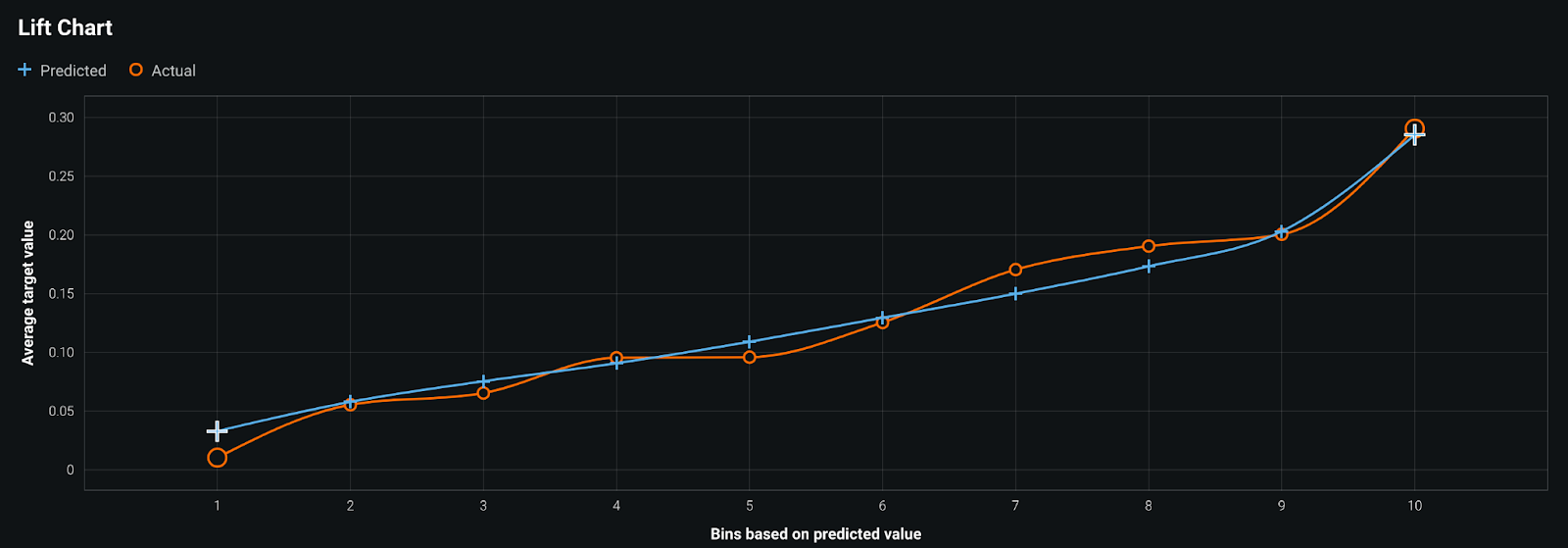
While model metrics help to quantify the model’s performance, it is by no means the only way of evaluating the overall quality of the model. To this end, a validator may also make use of a lift chart to see if the model they are reviewing is well calibrated for its objectives. For example, drawing upon the probability of default model discussed earlier in this post, a lift chart would be useful in determining if the model is able to discern between those applicants that pose the highest and least amount of credit risk for the financial institution. In the figure shown below, the predictions made by the model are compared against observed outcomes and rank ordered in increasing deciles based on the predicted value outputted by the model. It is clear in this case that the model is relatively well calibrated, as the actual outcomes observed align themselves closely with the predicted values. In other words, when the model predicts that an applicant is of high risk, we have correspondingly observed a higher rate of defaults (Bin 10 below), whereas we observe a much lower rate of defaults when the model predicts an applicant is at low risk (Bin 1). If, however, we had constructed a model that had a flat blue line for all the ordered deciles, it would have not been fit for its business objective, as the model had no means of discerning those applicants that are of high risk of defaulting versus those that weren’t.

Conclusion

Model validation is a critical component of the model risk management process, in which the proposed model is thoroughly tested to ensure that its design is fit for its objectives. In the context of modern machine learning methods, traditional validation approaches have to be adapted to make certain that the model is both conceptually sound and that its outcomes satisfy the necessary business requirements. 

In this post, we covered how DataRobot empowers the modeler and validator to gain a deeper understanding into model behavior by means of global and local feature importances, as well as providing feature effects plots to illustrate the direct relationship between model inputs and outputs. Because these techniques are model agnostic, they may be readily applied to sophisticated techniques employed today, without sacrificing on model explainability. In addition, by providing a host of model performance metrics and lift charts, the validator can be rest assured that the model is able to handle a wide range of data inputs appropriately and satisfy the business requirements for which it was created.

In the next post, we will continue our discussion on model validation by focusing on model monitoring. 

About the author

Harsh Patel

Data Platform Architect - Field CTO Office, Snowflake

Harsh Patel is a Customer-Facing Data Scientist at DataRobot. He leverages the DataRobot platform to drive the adoption of AI and Machine Learning at major enterprises in the United States, with a specific focus within the Financial Services Industry. Prior to DataRobot, Harsh worked in a variety of data-centric roles in both startups and major enterprises, where he had the opportunity to build many data products leveraging machine learning.
Harsh studied Physics and Engineering at Cornell University, and in his spare time enjoys traveling and exploring the parks in NYC.

Meet Harsh Patel