

No-Show Appointment Forecasting
This accelerator shows how to identify clients who are likely to miss appointments ("no-shows") and take action to prevent that from happening.
Request a DemoMany people are guilty of having cancelled a doctor’s appointment. However, although cancelling an appointment does not seem too disastrous from the patient’s point of view, no-shows cost outpatient health centres a staggering 14% of anticipated daily revenue (JAOA).
Missed appointments trickle into lower utilization rates for not only doctors and nurses but also the overhead costs required to run outpatient centres. In addition, patients missing their appointments risk facing poorer health outcomes as they are unable to access timely care.
While outpatient centres employ solutions such as calling patients ahead of time, these high touch resources investments are often not prioritized for patients with the highest risk of no-shows. Low touch solutions such as automated texts are effective tools for mass reminders but do not offer necessary personalization for patients at the highest risk of no-shows.
Use case type: Health Care, No-show forecasting
Complexity: Business analyst
Strategy: Identify clients likely to skip appointments (“no-shows”) and take action to prevent that from happening
How AI helps: Improve execution performance and demonstrate the best execution
Business drivers: Grow revenue, increase customer LTV, and increase customer satisfaction
Desired outcomes:
- Prevent no-shows
- Optimally target responses
- Reduce costs from missed appointments
- Add revenue from booking more appointments
Metrics and KPIs:
- Current no-show rate. Roughly 5% of all appointments are “no-show”.
- Cost of missed visit. On average, a missed visit costs the health care provider $150 per missed appointment.
Model usage: Rank order patients based on P(no-show) to prevent loss of revenue and potentially to overbook visits to prevent down-time.
Sample datasets
Solution value
AI enables your practice management staff to predict in advance which patients are likely to miss their appointments. By learning from historical data to uncover patterns related to no-shows, AI also provides your outpatient staff members with the top reasons why patients are likely to miss their appointments. These predictions and their explanations help your staff understand how various factors, such as a patient’s distance from a clinic and the days they needed to wait for their appointments, influence their risk of no-shows. Based on these predictions and insights, outpatient staff members can focus their outreach on patients with the highest risk of no-shows and offer them with solutions such as rescheduling their appointments or providing them with transportation.
The primary opportunities that this use case addresses are outlined in the table below.
| Issue | Opportunity |
|---|---|
| Patient outcome | Patients suffer if they do not get the care they require. Ensuring attendance plays a critical role in patient health. |
| Revenue loss | A degree of certainty about an open booking slot allows for preemptive filling by:Standard over-booking.Using a “propensity for” model to contact an alternative patient. |
| Staffing inefficiency | Correct staffing levels improve both patient and employee satisfaction. |
Setup
Import libraries
In [1]:

# Install the shapely and datarobot libraries
!pip install shapely --quiet
#!pip install datarobot --quiet

import datetime as datetime
import json
import os

from IPython.display import HTML
import datarobot as dr
import matplotlib.pyplot as plt
import numpy as np
import pandas as pd
import requests
import shapely.geometry
import shapely.wkt
import yaml

%matplotlib inline
Prepare data
Shape
The dataset for this use case consists of patient visits (one row per visit). For best results, the data should cover two years of historical appointments. This time window should include a complete sample of your data, accounting for seasonality and other important factors like COVID. Sampling at the patient ID, instead of the appointment ID, should be done so all appointments for a particular patient are present.
Features
Your dataset should contain, minimally, the following features:
- Patient ID
- Binary classification target (
show/no-show,0/1,True/False, etc.) - Date/time of the scheduled appointment
- Date the appointment was made
- The number of days between the appointment and when it was scheduled
Other helpful features to include are:
- Distance between the patient and the clinic they are visiting
- Historical no-show rates for the patient
- Reason for visit
- Clinic they are visiting
- The doctor they are visiting
- The age of the patient
- The gender of the patient
- Other factors about the patient (hypertension, diabetes, alcholism, etc.)
Example data
This accelerator contains robust sample data that gives an example of what features one might need. The following sections will walk you through preparing typical data and adding features that will allow your model to perform better.
In [2]:

# Function definition for data used at prediction time


def data_prep_sample(sample_df):
    sample_df["Schedule Date"] = pd.to_datetime(sample_df["Schedule Date"])
    sample_df["Appointment Date"] = pd.to_datetime(sample_df["Appointment Date"])

    # calulate the schedule delta between scheduled day and appointment day. Empty out the time so we are just left with days
    sample_df["Appointment/Schedule Delta"] = (
        sample_df["Appointment Date"]
        - sample_df["Schedule Date"].apply(
            lambda t: t.replace(minute=0, hour=0, second=0, microsecond=0)
        )
    ).apply(lambda t: t.days)

    # Calculate a new column that is the distance between the neighborhood and the clinic
    sample_df["Distance"] = df.apply(
        lambda l: calcDistance(l["Neighborhood"], l["Clinic Location"]), axis=1
    )

    sample_df["Appointment Date"] = sample_df["Appointment Date"].apply(
        lambda l: str(l)
    )
    sample_df["Schedule Date"] = sample_df["Schedule Date"].apply(lambda l: str(l))

    return sample_df
In [3]:
# Load the dataset
df = pd.read_csv(
"https://s3.amazonaws.com/datarobot_public_datasets/ai_accelerators/no_show/no_show.csv"
)
df.info()
df.head(2)<class 'pandas.core.frame.DataFrame'>
RangeIndex: 80000 entries, 0 to 79999
Data columns (total 14 columns):
# Column Non-Null Count Dtype
--- ------ -------------- -----
0 no_show 80000 non-null bool
1 Patient ID 80000 non-null object
2 Appointment ID 80000 non-null object
3 Gender 80000 non-null object
4 Age 80000 non-null int64
5 Alcohol Consumption 80000 non-null object
6 Hypertension 80000 non-null bool
7 Diabetes 80000 non-null bool
8 Appointment Date 80000 non-null object
9 Schedule Date 80000 non-null object
10 Appointment Reason 80000 non-null object
11 Clinic Location 80000 non-null object
12 Specialty 80000 non-null object
13 Neighborhood 80000 non-null object
dtypes: bool(3), int64(1), object(10)
memory usage: 6.9+ MB| 0 | 1 | |
| no_show | FALSE | FALSE |
| Patient ID | 649e3901-e56b-41d9-b2d3-f61ce708a415 | 3028fd02-a20a-4233-ac16-b571dde4540c |
| Appointment ID | 659a5257-c2f0-4eda-a2bb-ebc4bd9ce4e4 | 7ae6e7f8-3788-48d2-9fbc-11114ec28bfe |
| Gender | F | F |
| Age | 43 | 37 |
| Alcohol Consumption | 5/week | 0/week |
| Hypertension | FALSE | FALSE |
| Diabetes | FALSE | TRUE |
| Appointment Date | 2021-01-14 10:30:00 | 2021-02-17 14:00:00 |
| Schedule Date | 2020-10-26 0:00:00 | 2021-01-25 0:00:00 |
| Appointment Reason | CHIROPRACT MANJ 3-4 REGIONS | OFFICE/OUTPATIENT VISIT EST |
| Clinic Location | Mission Bay | Mission Bay |
| Specialty | Human Performance Center | Endocrine, Diabetes & Pregnancy Program |
| Neighborhood | Russian Hill | Ocean View |
The sample data contains the following features:
- no_show: The target variable. True if the patient DID NOT show, False if they did.
- Patient ID: Unique identifier for the patient.
- Appointment ID: Unique identifier for the appointment.
- Gender: Gender of the patient.
- Age: Age of the patient.
- Alcohol consumption: A categorical variable representing alcohol consumption per week.
- Hypertension: True if the patient is hypertensive.
- Diabetes: True if the patient is diabetic.
- Appointment date: The date and time for the appointment.
- Schedule date: The scheduled date for the appointment.
- Appointment reason: A text field containing the reasons for the appointment.
- Clinic location: The location of the clinic. This example uses clinics in San Francisco.
- Specialty: The specialist the patient sees.
- Neighborhood: The neighborhood the patient lives in. This example uses patients in San Francisco.
Examine some interesting facts about the data using the following cell.
In [4]:
# Look at the percentage of rows that are historical records of no-shows
print("no_show:")
print(df["no_show"].value_counts(normalize=True))
# Look at the number of clinic locations
print()
print("Number of Clinic Locations: " + str(df["Clinic Location"].nunique()))
# Examine the number of neighborhoods the patients live in
print()
print("Number of Neighborhoods: " + str(df["Neighborhood"].nunique()))
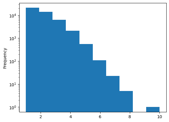
# Plot the number of appointments per patient
# Notice that most appointments are from patients that are new or have few historical appointments
print()
print("Patient ID:")
df["Patient ID"].value_counts().plot(kind="hist", logy=True)no_show:
False 0.959825
True 0.040175
Name: no_show, dtype: float64
Number of Clinic Locations: 9
Number of Neighborhoods: 37
Patient ID:
Out [4]:
<AxesSubplot:ylabel='Frequency'>
Looking at the feature list, it details a few interesting facts:
- no_show is the target variable. Roughly 4 percent of the visits were no-show visits.
- Patient ID represents the patient going to the appointment. The data contains multiple visits for one patient; therefore, you should choose the Group Partitioning method when loading the data into DataRobot.
- Clinic location is one of the nine clinic locations the patient visits.
- Neighborhood is one of the 37 neighborhoods in San Francisco that the patients live in. Calculating the distance between the patient neighborhood and the clinic would be extremely useful.
- Appointment date & schedule date are event dates (the date and the time in the case of appointment date). Engineering a feature that calculates the difference between these dates would also be useful.
Feature engineering
As mentioned above, engineering a few features will help the dataset tremendously. Specifically:
- With appointment date and the schedule date, calculate the real insight—the elapsed time, in days, between the two dates.
- The distance between where the patient lives and the clinic that is being visited.
- Historical no-show rates per patient.
There are many tools available to calculate these features. This example uses Python and Pandas to peform some simple calculations.
Appointment date and schedule date
In this section you calculate the difference, in days, between when the appointment was scheduled and when it occured. Add this difference as a feature so DataRobot can use it when building a model. This feature will be represented by the column Appointment/Schedule Delta.
In [5]:

# Change the schedule date and appointment date from strings to dates
df["Schedule Date"] = pd.to_datetime(df["Schedule Date"])
df["Appointment Date"] = pd.to_datetime(df["Appointment Date"])

# Calulate the schedule delta between the scheduled day and the appointment day
# Empty out the time so you are just left with days
df["Appointment/Schedule Delta"] = (
    df["Appointment Date"]
    - df["Schedule Date"].apply(
        lambda t: t.replace(minute=0, hour=0, second=0, microsecond=0)
    )
).apply(lambda t: t.days)
Distance to appointment
Next, calculate the distance between the two locations. This accelerator includes two additional datasets that will help to enrich the data:
- planning_neighborhoods.csv — The neighborhoods of San Francisco and their WKT geodata polygons.
- clinics.csv — The latitude and longitude of the clinics.
The following cell adds a new column, Distance. The distance is calculated as the geo distance between the centroid of the neighborhood the patient lives in to the location (latitude/longitude) of the clinic. The neighborhood and clinic names remain in the final dataset as they may be meaningful to the data.
In [6]:

# Create a map of neighborhood to the geometry of that neighborhood.
geo_df = pd.read_csv(
    "https://s3.amazonaws.com/datarobot_public_datasets/ai_accelerators/no_show/planning_neighborhoods.csv"
)
geo_df = geo_df.reset_index()
geo = {}

for index, row in geo_df.iterrows():
    geo[row["neighborho"]] = row["the_geom"]

# Create a map of clinic locations using the latitude and longitude of the clinic
clinic_df = pd.read_csv(
    "https://s3.amazonaws.com/datarobot_public_datasets/ai_accelerators/no_show/clinics.csv"
)
clinic_df = clinic_df.reset_index()
clinic = {}

for index, row in clinic_df.iterrows():
    clinic[row["name"]] = [row["lat"], row["long"]]
In [7]:
# Calculate the distance between the neighborhood and the clinic location
def calcDistance(neigh, loc):
# Load the geometry (WKT format)
p = shapely.wkt.loads(geo[neigh])
lat = clinic[loc][0]
long = clinic[loc][1]
# Convert the lat/long into a point
point = shapely.geometry.Point(long, lat)
# Calculate the distance between the centroid of the neighborhood and the point of the clinic
return p.distance(point)
# Add a new column that is the distance between the neighborhood and the clinic
df["Distance"] = df.apply(
lambda l: calcDistance(l["Neighborhood"], l["Clinic Location"]), axis=1
)Historical no-show rates
Next, load and calculate the historical no-show rates for each patient. For this example, assume that all historical data is stored in a CSV file keyed off of the Patient ID. (You would likely fetch these into a CSV or query a database.)
The historical data is included in no_show_historical.csv.
In [8]:

# Create a map of patient IDs to historical no show rates
hist_no_show_df = pd.read_csv(
    "https://s3.amazonaws.com/datarobot_public_datasets/ai_accelerators/no_show/no_show_historical.csv"
)
hist_no_show_df = hist_no_show_df.reset_index()
hist_no_show = {}

for index, row in hist_no_show_df.iterrows():
    hist_no_show[row["Patient ID"]] = row["no_show"]
In [9]:
# Add a new column that has the historical no show rate for that patient, or 0.0 if youe don't have the data
df["Hist No Show"] = df["Patient ID"].apply(lambda l: hist_no_show.get(l, 0.0))In [10]:
# fDrop the column "Appointment ID" as it will have no meaning in DataRobot
df = df.drop(columns=["Appointment ID"])Final dataset
The final dataset, with all features, is:
In [11]:

df.info()
pd.set_option("display.max_rows", 5)
display(df.loc[df["no_show"] == False])
display(df.loc[df["no_show"] == True])
<class 'pandas.core.frame.DataFrame'>
RangeIndex: 80000 entries, 0 to 79999
Data columns (total 16 columns):
# Column Non-Null Count Dtype
--- ------ -------------- -----
0 no_show 80000 non-null bool
1 Patient ID 80000 non-null object
2 Gender 80000 non-null object
3 Age 80000 non-null int64
4 Alcohol Consumption 80000 non-null object
5 Hypertension 80000 non-null bool
6 Diabetes 80000 non-null bool
7 Appointment Date 80000 non-null datetime64[ns]
8 Schedule Date 80000 non-null datetime64[ns]
9 Appointment Reason 80000 non-null object
10 Clinic Location 80000 non-null object
11 Specialty 80000 non-null object
12 Neighborhood 80000 non-null object
13 Appointment/Schedule Delta 80000 non-null int64
14 Distance 80000 non-null float64
15 Hist No Show 80000 non-null float64
dtypes: bool(3), datetime64[ns](2), float64(2), int64(2), object(7)
memory usage: 8.2+ MB| 0 | 1 | … | 79998 | 79999 | |
| no_show | FALSE | FALSE | … | FALSE | FALSE |
| Patient ID | 649e3901-e56b-41d9-b2d3-f61ce708a415 | 3028fd02-a20a-4233-ac16-b571dde4540c | … | 3570b112-021d-44da-be37-d2f76274ac90 | d066a33a-f9b8-40e9-9188-704e243202f8 |
| Gender | F | F | … | F | F |
| Age | 43 | 37 | … | 41 | 36 |
| Alcohol Consumption | 5/week | 0/week | … | 5/week | 5/week |
| Hypertension | FALSE | FALSE | … | FALSE | FALSE |
| Diabetes | FALSE | TRUE | … | FALSE | FALSE |
| Appointment Date | 2021-01-14 10:30:00 | 2021-02-17 14:00:00 | … | 2020-07-06 15:30:00 | 2021-09-08 10:30:00 |
| Schedule Date | 2020-10-26 | 2021-01-25 | … | 2020-06-17 | 2021-07-20 |
| Appointment Reason | CHIROPRACT MANJ 3-4 REGIONS | OFFICE/OUTPATIENT VISIT EST | … | ELECTROCARDIOGRAM REPORT | OFFICE/OUTPATIENT VISIT EST,LOCM 300-399mg/ml … |
| Clinic Location | Mission Bay | Mission Bay | … | Mission Bay | Laurel Village |
| Specialty | Human Performance Center | Endocrine, Diabetes & Pregnancy Program | … | Antenatal Testing Center | Primary Care at Laurel Village |
| Neighborhood | Russian Hill | Ocean View | … | Ocean View | Outer Mission |
| Appointment/Schedule Delta | 80 | 23 | … | 19 | 50 |
| Distance | 0.035496 | 0.072859 | … | 0.072859 | 0.051993 |
| Hist No Show | 0 | 0 | … | 0 | 0.26 |
| 89 | 153 | … | 79958 | 79961 | |
| no_show | TRUE | TRUE | … | TRUE | TRUE |
| Patient ID | bdf1e07e-2e60-44d7-8ccb-0a485a0bdb5b | 74152ac2-673f-4a12-9062-e01122d2af0f | … | f7f896bf-266f-42f0-acb8-9f1844c61cec | 715f74a8-325b-4b39-b28b-7722111abb58 |
| Gender | F | M | … | F | M |
| Age | 58 | 47 | … | 36 | 56 |
| Alcohol Consumption | 5/week | > 14/week | … | 0/week | 0/week |
| Hypertension | TRUE | FALSE | … | FALSE | FALSE |
| Diabetes | FALSE | FALSE | … | FALSE | FALSE |
| Appointment Date | 2021-05-14 15:45:00 | 2021-04-27 11:00:00 | … | 2020-10-02 16:00:00 | 2020-07-28 9:45:00 |
| Schedule Date | 2021-02-17 | 2021-02-01 | … | 2020-06-15 | 2020-03-17 |
| Appointment Reason | OFFICE/OUTPATIENT VISIT EST | SUBSEQUENT HOSPITAL CARE | … | Chest x-ray 2vw frontal&latl | OFFICE/OUTPATIENT VISIT EST,Ferumoxytol non-esrd |
| Clinic Location | Mount Zion | Mission Bay | … | Parnassus | Mount Zion |
| Specialty | High-Risk Skin Cancer Clinic | Human Performance Center | … | California Center for Pituitary Disorders | Pain Management Center |
| Neighborhood | Excelsior | Presidio | … | Lakeshore | Excelsior |
| Appointment/Schedule Delta | 86 | 85 | … | 109 | 133 |
| Distance | 0.054118 | 0.061707 | … | 0.028724 | 0.054118 |
| Hist No Show | 0 | 0.18 | … | 0.3 | 0.25 |
Connect to DataRobot
Read more about different options for connecting to DataRobot from the client.
In [12]:
# Create a client connection to DR
dr.Client()
Out [12]:

<datarobot.rest.RESTClientObject at 0x7f4a25907410>
Import data
The final dataset now needs to be loaded into DataRobot via the API. Alternatively, you can modify the code above to save the final dataset as a CSV and use it to create a project in DataRobot.
In [13]:

# Write out the final version of the dataset
ct = datetime.datetime.now()
file_name = f"no_show_enriched_{int(ct.timestamp())}.csv"

dataset = dr.Dataset.create_from_in_memory_data(df)
dataset.modify(name=file_name)

dataset

# df.to_csv("./" + file_name, index=False)
Out [13]:
Dataset(name='no_show_enriched_1686808642.csv', id='648aa84ae0838f6f81bbcb2b')
Modeling
Create a DataRobot project
Now it is time to create a project in DataRobot. There are a couple of ways this could be done. It could be loaded using the UI or, as the following code shows, it can be done using the DataRobot API.
Note: Choose the following settings from the UI if you are creating the project manually.
- Choose the feature no_show as the target feature.
- Choose Group partitioning (Advanced options > Partitioning group) and set the Group ID Feature to Patient ID.
- Create a new feature list that excludes Approval Date and Schedule Date to control which features are used in model creation. Specifically, the list will keep the components of the Approval Date and Schedule Date, but does not keep the dates themselves.
The following code creates the project in DataRobot with the correct settings.
In [14]:

# Create the project
ct = datetime.datetime.now()
project_name = f"no_show_enriched_{int(ct.timestamp())}"

project = dataset.create_project(project_name=project_name)
In [15]:
# Now create a new feature list that contains all of the "Informative Features" in the project
# This feature list will contain all derived features DataRobot created for you
flists = project.get_featurelists()
flist = next(x for x in flists if x.name == "Informative Features")
# You don't want dates in the feature list, just the components created by DataRobot
new_features = [
x for x in flist.features if x not in ["Appointment Date", "Schedule Date"]
]
# Create the new feature list in DataRobot
fl = project.create_featurelist(name="No Dates", features=new_features)
# Uncomment the next line to print out a link that can be used to access the project UI in DataRobot
# display(HTML(f'At this point you can <a target="_blank" rel="noopener noreferrer" href="https://app.datarobot.com/projects/{project.id}/eda">click into the project</a> and look at the features. Notice the new feature list we created.'))Start Autopilot
Next, set your project options, target, partitioning method, and feature list. Then you will start Autopilot and wait for it to finish.
In [16]:

group_cv = dr.GroupCV(20, 5, ["Patient ID"])

project.analyze_and_model(
    # Set the target as the no_show column
    target="no_show",
    # Don't limit the worker count
    worker_count="-1",
    # Group partition on the Patient ID column
    partitioning_method=group_cv,
    mode=dr.AUTOPILOT_MODE.QUICK,
    # Set the feature list that was created above
    featurelist_id=fl.id,
)

# Uncomment the next line to print out a link that can be used to access the project UI in DataRobot
# display(HTML(f'Now you can navigate to the models page of the new project or <a target="_blank" rel="noopener noreferrer" href="https://app.datarobot.com/projects/{project.id}/models">click this link</a>'))

project.wait_for_autopilot(verbosity=0)
Navigate to project in the UI
Once the project is created and Autopilot has finished, you should navigate to the project in the UI. Use the following cell to retrieve the name of the project.
In [17]:

print(project_name)
no_show_enriched_1686808709
Analyze models
Exploratory Data Analysis
Navigate to the Data tab to learn more about your data.
- Click each feature to see a histogram that represents the relationship of the feature with the target.
- The Feature Associations tab visualizes clusters of related columns.
Leaderboard
You can click on the Models tab to view the Leaderboard and see generated models as they build.
From the Leaderboard, click on any model to reveal the blueprint—the pipeline of preprocessing steps, modeling algorithms, and post-processing steps. Autopilot will continue building models until it selects the best predictive model for the specified target feature. This model is at the top of the Leaderboard, marked with the Recommended for Deployment badge.
Please see the DataRobot documentation for more information.
Evaluation
After you have clicked on a model, under the Evaluate tab, view the ROC Curve. The information here can be used to calculate the ROI of the solution. ROI is directly related to how you operationalize the model.
For this use case, the goal is to build a call list that results in changing the outcome for patients that might not have shown up, while minimizing the number of people called that would have attended without prompting. You can do so by assigning payoffs for the True Positives and False Positives of the payoff matrix.
- Choose Add Payoff in the Matrix pane and enter values for True Positive and False Positive. For example: TP=
$120and FP=-$5 - For metrics, select False Positive Rate (Fallout), Positive Predictive Value (Precision), and Average Profit.
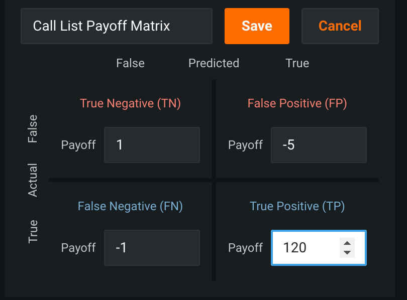
Choosing a True Positive payout of $120 indicates saving $120 for every patient that shows up once called. A false positive payout of -$5 reflects the cost of $5 to make the call.
The decision boundary suggested for max profit is not practical because almost 20% of appointments (the Fallout rate) would require a personalized reminder. Adjust where on the curve to set that target for the model.
- Click on different points of the ROC curve to see what the recall rate looks like for Fallout values of 5% and 10%.
- At 5%, the precision is roughly 27% and average profit is roughly $3
- At 10%, the precision is roughly 21% and the average profit is roughly $3.40
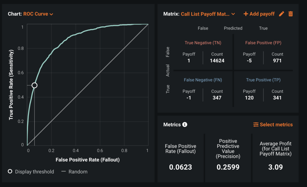
Choosing a Fallout of roughly 6% gives a proffit of roughly $3 which is in range for this use case.
Insights
There are many ways within DataRobot to veiw insights into why a patient might not show. Below are the most relavent for this use case, all found under the Understand tab of the Leaderboard.
Feature Impact
Feature Impact is one way to view which features are driving model decisions. A large impact means model performance deteriorates significantly when this feature is removed. Features with low impact may still contribute to the model.
For this use case Hist No Show, Appointment/Schedule Delta, Distance, Appointment Reason, and Alcohol Consumption are the most impactful features.
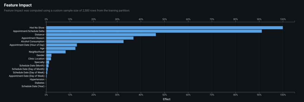
One would agree that these features are likely the features that would impact if someone will show up for an appointment. For example, if that person has a history of not showing up then it makes sense to predict they won’t in the future.
See the DataRobot documentation for more information on how to interpret this section.
Feature Effects
Feature Effects shows how a model is effected when a the value of a feature changes. For this use case:
- For
Appointment Delta, a larger disparity between dates increases the likelihood of a no-show. - For
Distance, further distance from the clinic increases the likelihood of a no-show.
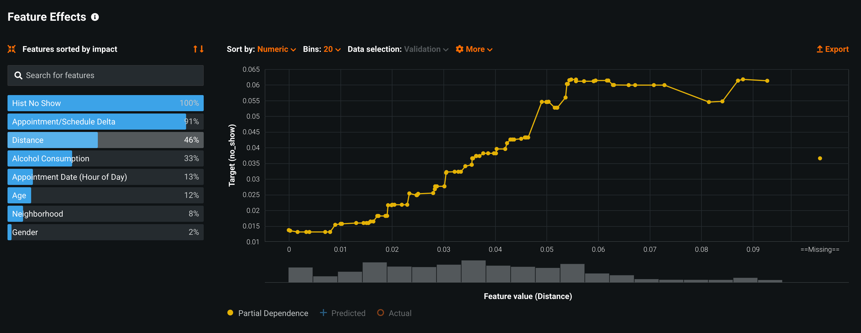
The image above is showing the feature effects that the Distance feature has on results. Notice that the farther away a patient is from the clinic the less likely they are to show up for their appointment.
See the DataRobot documentation for more information on how to interpret this section.
Prediction Explanations
Prediction Explanations provide the drivers behind each prediction.
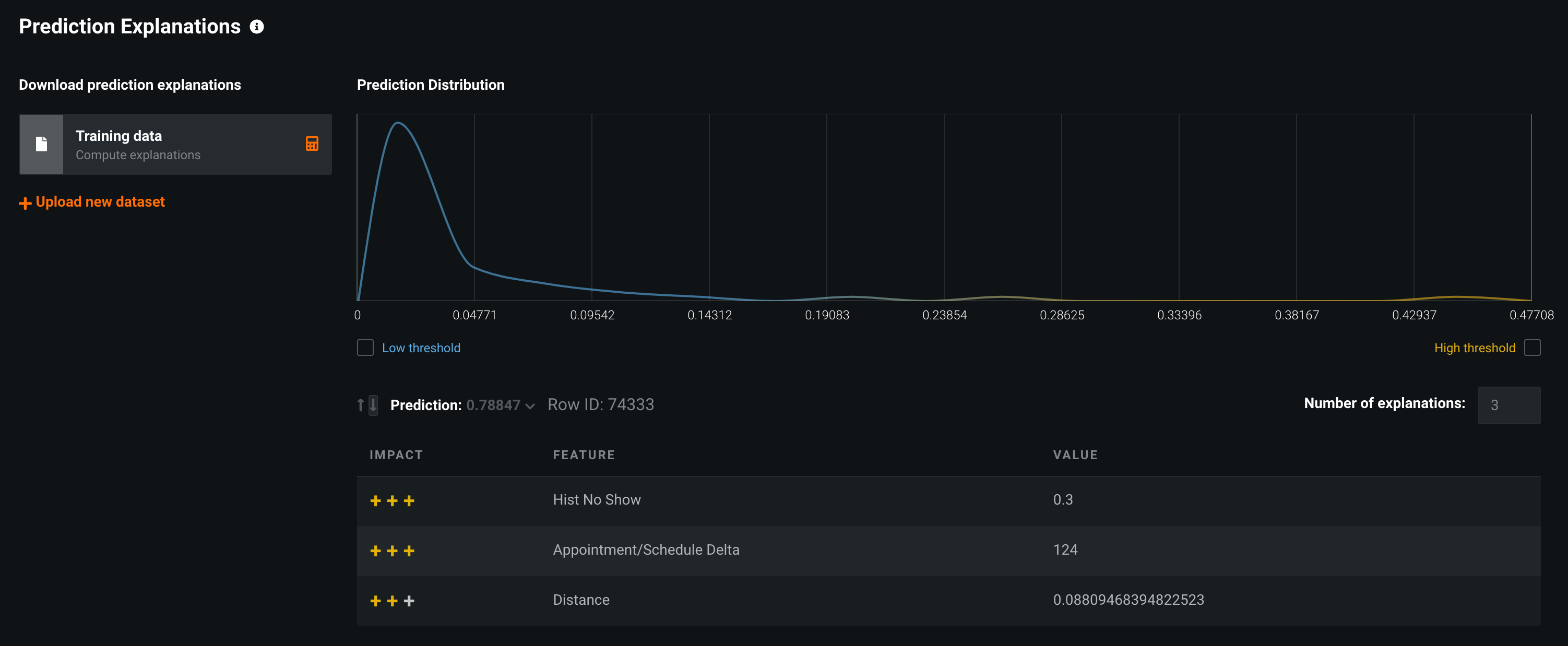
For the row in the image above, Hist No Show, Appointment/Schedule Delta, and Distance are the features contributing most to the reason the model predicts this row to be a no-show.
See the DataRobot documentation for more information on how to interpret this section.
Word Cloud
The word cloud allows you to explore how text fields affect predictions.
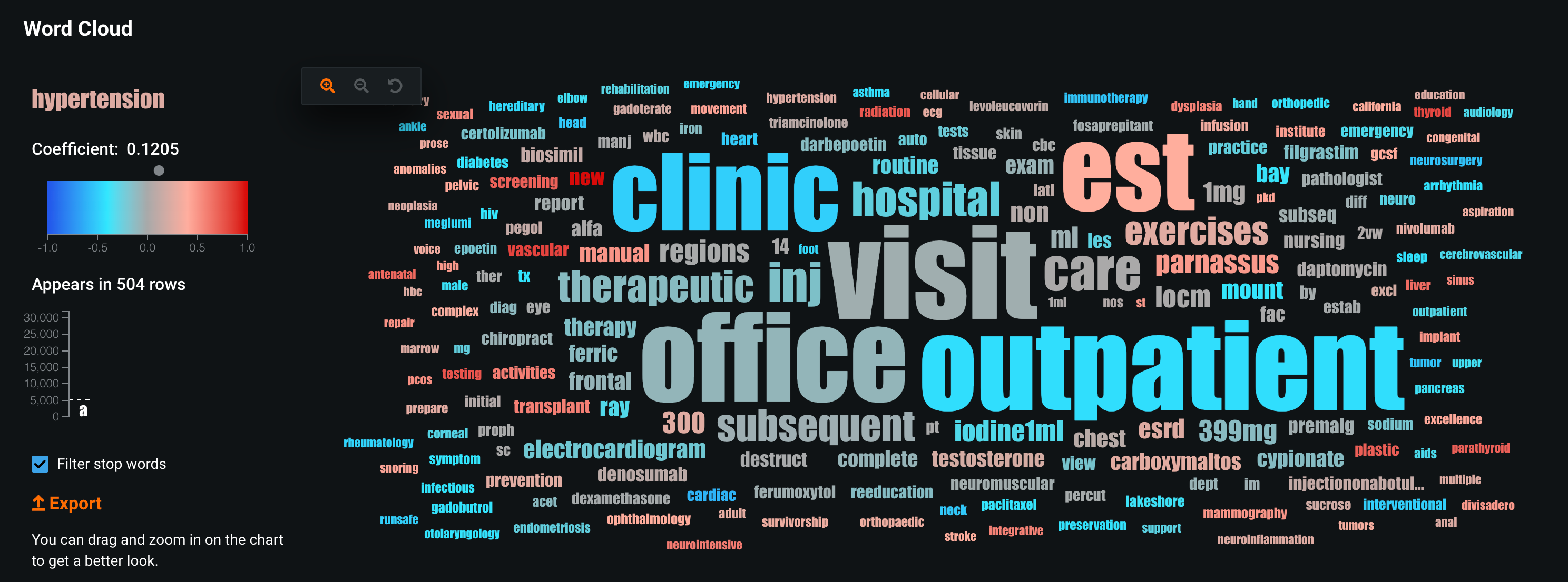
In this use case, patients that have new in the reason for the visit are the least likely to show up.
See the DataRobot documentation for more information on how to interpret this section.
Compliance
If available for your organization, from the Compliance tab you can compile model development documentation, in MS Word format, that can be used for regulatory validation.
See the DataRobot documentation for more information on how to interpret this section.
Make predictions
Once you understand and have selected a model, it can be deployed. This example deploys the recommended model (marked with a badge) from the Leaderboard. You can deploy in the UI from the model’s Predict > Deploy tab or using Python, as shown below.
In [18]:

# Get the recommended model
model_depl = dr.ModelRecommendation.get(project.id).get_model()

pred_serv_id = dr.PredictionServer.list()[0].id
deployment = dr.Deployment.create_from_learning_model(
    model_id=model_depl.id,
    label=f"{project_name}_depl",
    default_prediction_server_id=pred_serv_id,
)
In [19]:
deployment.update_association_id_settings(
column_names=["Appointment ID"], required_in_prediction_requests=True
)
deployment.update_drift_tracking_settings(True, True)In [20]:
# Generate explanations
# To compute Feature Impact:
feature_impacts = model_depl.get_or_request_feature_impact()
# To initialize Prediction Explanations:
pei_job = dr.PredictionExplanationsInitialization.create(project.id, model_depl.id)
pei_job.wait_for_completion()The following lines of code predict no-shows for January. It will generate a list of patients that should be called for that month.
You can read more about configuring batch predictions in DataRobot’s Python client documentation.
In [21]:

# First set the display options
pd.set_option("display.max_rows", 25)
pd.set_option("display.max_columns", None)

df_scoring_csv = pd.read_csv(
    "https://s3.amazonaws.com/datarobot_public_datasets/ai_accelerators/no_show/jan_sample.csv"
)
df_scoring = data_prep_sample(df_scoring_csv)

job, results_df = dr.BatchPredictionJob.score_pandas(
    deployment, df_scoring, max_explanations=3
)

results_df.loc[results_df["no_show_PREDICTION"] == True].head()
Streaming DataFrame as CSV data to DataRobot
Created Batch Prediction job ID 648aabdf32e7c4333cbb704c
Waiting for DataRobot to start processing
Job has started processing at DataRobot. Streaming results.| 6 | 33 | 121 | 177 | |
| Unnamed: 0 | 6 | 33 | 121 | 177 |
| Patient ID | bf978545-1275-45c2-8ed9-f69ae156771c | 806f594a-997c-4278-8544-7dbdd8a46fc2 | 717442f1-e0ba-4f27-a0ce-cc1ff96de253 | c4cc388f-0b62-4339-b8ad-06146036114e |
| Appointment ID_x | 1eb56386-3499-471e-93f8-98d663a9bd1d | 440d8da1-f69e-4d1f-b75f-46a318a4c01b | bd2dd6b6-0b35-444e-92fa-20c1f7595ae9 | a836bf05-aca4-4d90-8e53-bf03cbf3f7bb |
| Gender | F | M | M | M |
| Age | 17 | 55 | 41 | 42 |
| Alcohol Consumption | 0/week | > 14/week | > 14/week | > 14/week |
| Hypertension | FALSE | FALSE | FALSE | FALSE |
| Diabetes | FALSE | FALSE | FALSE | FALSE |
| Appointment Date | 2022-01-31 8:30:00 | 2022-01-06 9:30:00 | 2022-01-19 8:00:00 | 2022-01-04 8:00:00 |
| Schedule Date | 2021-08-03 0:00:00 | 2021-08-17 0:00:00 | 2021-07-19 0:00:00 | 2021-08-06 0:00:00 |
| Appointment Reason | OFFICE/OUTPATIENT VISIT NEW,Daptomycin injecti… | THERAPEUTIC EXERCISES,Inj testosterone cypionate | THERAPEUTIC EXERCISES | OFFICE/OUTPATIENT VISIT EST,Paclitaxel injection |
| Clinic Location | Parnassus | Mount Zion | Parnassus | Mount Zion |
| Specialty | Infusion Center | Mammography Screening | Neuro/Psych Sleep Clinic | Osher Center for Integrative Medicine |
| Neighborhood | Outer Mission | Parkside | Outer Richmond | Glen Park |
| Hist No Show | 0.25 | 0.36 | 0.17 | 0.21 |
| Appointment/Schedule Delta | 181 | 142 | 184 | 151 |
| Distance | 0.051588 | 0.059132 | 0.09621 | 0.053679 |
| no_show_True_PREDICTION | 0.508578 | 0.634147 | 0.668767 | 0.558122 |
| no_show_False_PREDICTION | 0.491422 | 0.365853 | 0.331233 | 0.441878 |
| no_show_PREDICTION | TRUE | TRUE | TRUE | TRUE |
| THRESHOLD | 0.5 | 0.5 | 0.5 | 0.5 |
| POSITIVE_CLASS | TRUE | TRUE | TRUE | TRUE |
| EXPLANATION_1_FEATURE_NAME | Appointment Reason | Appointment/Schedule Delta | Appointment/Schedule Delta | Appointment/Schedule Delta |
| EXPLANATION_1_STRENGTH | 1.337003 | 1.414675 | 1.415882 | 1.329059 |
| EXPLANATION_1_ACTUAL_VALUE | OFFICE/OUTPATIENT VISIT NEW,Daptomycin injecti… | 142 | 184 | 151 |
| EXPLANATION_1_QUALITATIVE_STRENGTH | +++ | +++ | +++ | +++ |
| EXPLANATION_2_FEATURE_NAME | Hist No Show | Hist No Show | Hist No Show | Hist No Show |
| EXPLANATION_2_STRENGTH | 1.235433 | 1.249752 | 1.256081 | 1.215514 |
| EXPLANATION_2_ACTUAL_VALUE | 0.25 | 0.36 | 0.17 | 0.21 |
| EXPLANATION_2_QUALITATIVE_STRENGTH | +++ | +++ | +++ | +++ |
| EXPLANATION_3_FEATURE_NAME | Appointment/Schedule Delta | Alcohol Consumption | Alcohol Consumption | Alcohol Consumption |
| EXPLANATION_3_STRENGTH | 1.17557 | 1.017528 | 0.931668 | 0.961447 |
| EXPLANATION_3_ACTUAL_VALUE | 181 | > 14/week | > 14/week | > 14/week |
| EXPLANATION_3_QUALITATIVE_STRENGTH | +++ | ++ | ++ | ++ |
| DEPLOYMENT_APPROVAL_STATUS | APPROVED | APPROVED | APPROVED | APPROVED |
| Appointment ID_y | 1eb56386-3499-471e-93f8-98d663a9bd1d | 440d8da1-f69e-4d1f-b75f-46a318a4c01b | bd2dd6b6-0b35-444e-92fa-20c1f7595ae9 | a836bf05-aca4-4d90-8e53-bf03cbf3f7bb |
Each table above is showing patients who possibly will not show up to their next appointment. These results can be used in a separate application or integreting with another system. Either way the code above shows how that call list can be generated.
Functionality overview
The following DataRobot functionality was employed in this use case:
| FEATURE | BENEFIT |
|---|---|
| Group Partitioning | Used to group the input data by patient ID. |
| Feature Lists | Used to remove dates from the input features for DataRobot. |
| Profit Curve | Helps to optimize the cost of a bad prediction vs. the value of a good one. |
| Prediction Explanations | Generates explanations that contribute to each score. |
| Word Cloud | Helps to explain what visit codes contribute to no-show appointments. |
Get Started with No-Show Forecasting

Explore more AI Accelerators
-
HorizontalObject Classification on Video with DataRobot Visual AI
This AI Accelerator demonstrates how deep learning model trained and deployed with DataRobot platform can be used for object detection on the video stream (detection if person in front of camera wears glasses).
Learn More -
HorizontalPrediction Intervals via Conformal Inference
This AI Accelerator demonstrates various ways for generating prediction intervals for any DataRobot model. The methods presented here are rooted in the area of conformal inference (also known as conformal prediction).
Learn More -
HorizontalReinforcement Learning in DataRobot
In this notebook, we implement a very simple model based on the Q-learning algorithm. This notebook is intended to show a basic form of RL that doesn't require a deep understanding of neural networks or advanced mathematics and how one might deploy such a model in DataRobot.
Learn More -
HorizontalDimensionality Reduction in DataRobot Using t-SNE
t-SNE (t-Distributed Stochastic Neighbor Embedding) is a powerful technique for dimensionality reduction that can effectively visualize high-dimensional data in a lower-dimensional space.
Learn More