End-to-End Time Series Demand Forecasting Workflow

In this first installment of a three-part series on demand forecasting, this accelerator provides the building blocks for a time-series experimentation and production workflow.

Build with Free Trial

Time series forecasting in DataRobot has a huge suite of tools and approaches to handle highly complex multiseries problems. These include:

• Automatic feature engineering and creation of lagged variables across multiple data types, as well as training dataset creation
• Diverse approaches for time series modeling with text data, learning from cross-series interactions, and scaling to hundreds or thousands of series
• Feature generation from an uploaded calendar of events file specific to your business or use case
• Automatic backtesting controls for regular and irregular time series
• Training dataset creation for an irregular series via custom aggregations
• Segmented modeling, hierarchical clustering for multi-series models, text support, and ensembling
• Periodicity and stationarity detection and automatic feature list creation with various differencing strategies
• Cold start modeling on series with limited or no history
• Insights for models

This notebook serves as an introduction to that diverse functionality via the Python SDK. Subsequent notebooks in this series will dig deeper into the nuance of seeing data drift in production, handling cold-start series, and deploying a web-based application for what-if analysis for promotion planning. As such, this notebook provides a framework to inspect and handle common data and modeling challenges, identifying common pitfalls in real-life time series data, and leaving it to the reader to dig deeper on specific issues. The dataset consists of 50 skus across many stores over a 2 year period with varying series history, typical of a business releasing and removing products over time.

DataRobot will be used for the model training, selection, deployment, and making predictions. Snowflake will work as a datasource for both training and testing, and as a storage to write predictions back. This workflow, however, applies to any data source, e.g. Redshift, S3, Big Query, Synapse, etc. For examples of data loading from other environemnts, check out the other end-to-end examples in this Git Repo.

The following steps are covered:

• Ingesting the data from Snowflake into AI Catalog within DataRobot
• Running a new DataRobot project
• Getting the insights from the top model
• Deploying the recommended model
• Defining and running a job to make predictions and write them back into Snowflake

Setup

Optional: Import public demo data

For this workflow, you can download publicly available datasets (training, scoring, and calendar data) from DataRobot’s S3 bucket to your database or load into your DataRobot instance.

If you are using Snowflake, you will need to update the fields below with your Snowflake information. Data will be loaded and created in your Snowflake instance. You will also need the following files found in the same repo as this notebook:

• dr_utils.py
• datasets.yaml

Once you are done with this notebook, remember to delete the data from your Snowflake instance.

In [1]:

# requires Python 3.8 or higher
from dr_utils import prepare_demo_tables_in_db

Fill out the credentials for your Snowflake instance. You will need write access to a database.

In [2]:

db_user = "your_username"  # Username to access Snowflake database
db_password = "your_password"  # Password
account = "account"  # Snowflake account identifier
db = "YOUR_DB_NAME"  # Database to Write_To
warehouse = "YOUR_WAREHOUSE"  # Warehouse
schema = "YOUR_SCHEMA"  # Schema

Use the util function to pull the data from DataRobot’s public S3 and import into your Snowflake instance.

In [3]:

response = prepare_demo_tables_in_db(
    db_user=db_user,
    db_password=db_password,
    account=account,
    db=db,
    warehouse=warehouse,
    schema=schema,
)

******************************
table: ts_demand_forecasting_train

	0	1	2	3	4
STORE_SKU	store_130_SKU_120931082	store_130_SKU_120931082	store_130_SKU_120931082	store_130_SKU_120931082	store_130_SKU_120931082
DATE	2019-05-06	2019-05-13	2019-05-20	2019-05-27	2019-06-03
UNITS	388	318	126	285	93
UNITS_MIN	44	37	13	23	10
UNITS_MAX	69	62	23	65	20
UNITS_MEAN	55.428571	45.428571	18	40.714286	13.285714
UNITS_STD	8.182443	8.079958	3.91578	14.067863	3.352327
TRANSACTIONS_SUM	243	210	118	197	87
PROMO_MAX	1	1	0	1	0
PRICE_MEAN	44.8	44.8	44.8	44.8	44.8
STORE	store_130	store_130	store_130	store_130	store_130
SKU	SKU_120931082	SKU_120931082	SKU_120931082	SKU_120931082	SKU_120931082
SKU_CATEGORY	cat_1160	cat_1160	cat_1160	cat_1160	cat_1160

info for  ts_demand_forecasting_train
<class 'pandas.core.frame.DataFrame'>
RangeIndex: 8589 entries, 0 to 8588
Data columns (total 13 columns):
 #   Column            Non-Null Count  Dtype  
---  ------            --------------  -----  
 0   STORE_SKU         8589 non-null   object 
 1   DATE              8589 non-null   object 
 2   UNITS             8589 non-null   float64
 3   UNITS_MIN         8589 non-null   float64
 4   UNITS_MAX         8589 non-null   float64
 5   UNITS_MEAN        8589 non-null   float64
 6   UNITS_STD         8589 non-null   float64
 7   TRANSACTIONS_SUM  8589 non-null   float64
 8   PROMO_MAX         8589 non-null   float64
 9   PRICE_MEAN        8589 non-null   float64
 10  STORE             8589 non-null   object 
 11  SKU               8589 non-null   object 
 12  SKU_CATEGORY      8589 non-null   object 
dtypes: float64(8), object(5)
memory usage: 872.4+ KB
None
writing ts_demand_forecasting_train to snowflake from:  https://s3.amazonaws.com/datarobot_public_datasets/ai_accelerators/ts_demand_forecasting_train.csv
******************************
table: ts_demand_forecasting_scoring

	0	1	2	3	4
STORE_SKU	store_130_SKU_120931082	store_130_SKU_120931082	store_130_SKU_120931082	store_130_SKU_120931082	store_130_SKU_120931082
DATE	2022-07-04	2022-07-11	2022-07-18	2022-07-25	2022-08-01
UNITS	70	89	90	77	85
UNITS_MIN	7	5	10	4	6
UNITS_MAX	13	19	18	20	26
UNITS_MEAN	10	12.714286	12.857143	11	12.142857
UNITS_STD	2.581989	5.936168	3.132016	5	6.466028
TRANSACTIONS_SUM	65	84	85	67	82
PROMO_MAX	0	0	0	0	0
PRICE_MEAN	22.8	22.8	22.8	22.8	22.8
STORE	store_130	store_130	store_130	store_130	store_130
SKU	SKU_120931082	SKU_120931082	SKU_120931082	SKU_120931082	SKU_120931082
SKU_CATEGORY	cat_1160	cat_1160	cat_1160	cat_1160	cat_1160

info for  ts_demand_forecasting_scoring
<class 'pandas.core.frame.DataFrame'>
RangeIndex: 1050 entries, 0 to 1049
Data columns (total 13 columns):
 #   Column            Non-Null Count  Dtype  
---  ------            --------------  -----  
 0   STORE_SKU         1050 non-null   object 
 1   DATE              1050 non-null   object 
 2   UNITS             850 non-null    float64
 3   UNITS_MIN         850 non-null    float64
 4   UNITS_MAX         850 non-null    float64
 5   UNITS_MEAN        850 non-null    float64
 6   UNITS_STD         850 non-null    float64
 7   TRANSACTIONS_SUM  850 non-null    float64
 8   PROMO_MAX         1050 non-null   float64
 9   PRICE_MEAN        850 non-null    float64
 10  STORE             1050 non-null   object 
 11  SKU               1050 non-null   object 
 12  SKU_CATEGORY      1050 non-null   object 
dtypes: float64(8), object(5)
memory usage: 106.8+ KB
None
writing ts_demand_forecasting_scoring to snowflake from:  https://s3.amazonaws.com/datarobot_public_datasets/ai_accelerators/ts_demand_forecasting_scoring.csv
******************************
table: ts_demand_forecasting_calendar
date	event_type
0	2017-01-01	New Year's Day
1	2017-01-02	New Year's Day (Observed)
2	2017-01-16	Martin Luther King, Jr. Day
3	2017-02-20	Washington's Birthday
4	2017-05-29	Memorial Day
info for  ts_demand_forecasting_calendar
<class 'pandas.core.frame.DataFrame'>
RangeIndex: 81 entries, 0 to 80
Data columns (total 2 columns):
 #   Column      Non-Null Count  Dtype 
---  ------      --------------  ----- 
 0   date        81 non-null     object
 1   event_type  81 non-null     object
dtypes: object(2)
memory usage: 1.4+ KB
None
writing ts_demand_forecasting_calendar to snowflake from:  https://s3.amazonaws.com/datarobot_public_datasets/ai_accelerators/ts_demand_forecasting_calendar.csv

Import libraries

In [4]:

from datetime import datetime as dt
from platform import python_version

import datarobot as dr
import dr_utils as dru
import pandas as pd

print("Python version:", python_version())
print("Client version:", dr.__version__)

Python version: 3.9.7
Client version: 3.0.2

Connect to DataRobot

1. In DataRobot, navigate to Developer Tools by clicking on the user icon in the top-right corner. From here you can generate a API Key that you will use to authenticate to DataRobot. You can find more details on creating an API key in the DataRobot documentation.
2. Determine your DataRobot API Endpoint. The API endpoint is the same as your DataRobot UI root. Replace {datarobot.example.com} with your deployment endpoint.API endpoint root: https://{datarobot.example.com}/api/v2For users of the AI Cloud platform, the endpoint is https://app.datarobot.com/api/v2
3. After obtaining your API Key and endpoint, there are several options to connect to DataRobot. This notebook uses option B.A. Create a .yaml file and refer to it in the code:

A. Create a .yaml file and refer to it in the code:

 - .yaml config file example:

 ```yaml
 endpoint: 'https://{datarobot.example.com}/api/v2'
 token: 'YOUR_API_KEY'


  ```

 - Code to connect:

 ```python
 dr.Client(config_path = "~/.config/datarobot/drconfig.yaml")


 ```

B. Set environment variables in the UNIX shell

 ```shell
 export DATAROBOT_ENDPOINT=https://{datarobot.example.com}/api/v2
 export DATAROBOT_API_TOKEN=YOUR_API_KEY


 ```
 - Code to connect:

 ```python
 dr.Client()


 ```

C. Embed in the code

 ```python
 dr.Client(endpoint='https://{datarobot.example.com}/api/v2', token='YOUR_API_KEY')

 ```

In [5]:

# Instantiate the DataRobot connection

DATAROBOT_API_TOKEN = ""  # Get this from the Developer Tools page in the DataRobot UI
# Endpoint - This notebook uses the default endpoint for DataRobot Managed AI Cloud (US)
DATAROBOT_ENDPOINT = "https://app.datarobot.com/"  # This should be the URL you use to access the DataRobot UI

client = dr.Client(
    token=DATAROBOT_API_TOKEN,
    endpoint=DATAROBOT_ENDPOINT,
    user_agent_suffix="AIA-E2E-TS-24",  # Optional but helps DataRobot improve this workflow
)

dr.client._global_client = client

Data preparation

In general, data preparation consists of several broadly defined steps:

• Explanatory data analysis
• Training data selection
• Data preparation itself based on the previous steps

Depending on the use case some of these steps can be skipped or additional business related steps may be necessary.

In this section you should define:

• The unit of analysis: every SKU sales or the whole store sales
• Observation frequency:
  • If the data is at the transaction level, you should aggregate to some regular timestamp, such as hour or day;
  • Sometimes the data provided is already aggregated, but it has a lot of missing dates. Or, from the business perspective, you may need predictions with lower resolution (e.g., weekly or monthly instead of hourly or daily).

The dataset should contain at least the following columns:

• Date
• Series ID: SKU, Store, Store – SKU combination
• Target

Additionally, the calendar file can be specified. DataRobot will automatically create features based on the calendar events (such as “days to next event” ).

Define variables

In [6]:

date_col = "DATE"
series_id = "STORE_SKU"
target = "UNITS"

Configure a data connection

DataRobot supports connections to a wide variety of databases through AI Catalog, allowing repeated access to the database as an AI Catalog Data Store. You can find the examples in the DataRobot documentation.

Credentials for the connection to your Data Store can be securely stored within DataRobot. They will be used during the dataset creation in the AI Catalog, and can be found under the Data Connections tab in DataRobot.

If you don’t have credentials and a datastore created, uncomment and run the cell below.

In [ ]:

# # Find the driver ID from name
# Can be skipped if you have the ID - showing the code here for completeness
# for d in dr.DataDriver.list():
#     if d.canonical_name in 'Snowflake (3.13.9 - recommended)':
#         print((d.id, d.canonical_name))

# # Create a datastore and datastore ID
# data_store = dr.DataStore.create(data_store_type='jdbc', canonical_name='Snowflake Demo DB', driver_id='626bae0a98b54f9ba70b4122', jdbc_url= db_url)
# data_store.test(username=db_user, password=db_password)

# # Create and store credentials to allow the AI Catalog access to this database
# # These can be found in the Data Connections tab under your profile in DataRobot
# cred = dr.Credential.create_basic(name='test_cred',user=db_user, password=db_password,)

Use the snippet below to find a credential and a data connection (AKA a datastore).

In [ ]:

creds_name = "your_stored_credential"
data_store_name = "your_datastore_name"

credential_id = [
    cr.credential_id for cr in dr.Credential.list() if cr.name == creds_name
][0]
data_store_id = [
    ds.id for ds in dr.DataStore.list() if ds.canonical_name == data_store_name
][0]

Use the snippet below to create or get an existing data connection based on a query and upload a training dataset into the AI Catalog.

In [12]:

data_source_train, dataset_train = dru.create_dataset_from_data_source(
    data_source_name="ts_training_data",
    query=f'select * from {db}.{schema}."ts_demand_forecasting_train";',
    data_store_id=data_store_id,
    credential_id=credential_id,
)

new data source: DataSource('ts_training_data')

Use the following snippet to create or get an existing data connection based on a query and upload a calendar dataset into the AI Catalog.

In [14]:

data_source_calendar, dataset_calendar = dru.create_dataset_from_data_source(
    data_source_name="ts_calendar",
    query=f'select * from {db}.{schema}."ts_demand_forecasting_calendar";',
    data_store_id=data_store_id,
    credential_id=credential_id,
)

new data source: DataSource('ts_calendar')

The following snippet is optional and can be used to get data to investigate before modeling.

In [15]:

df = dataset_train.get_as_dataframe()
df[date_col] = pd.to_datetime(df[date_col], format="%Y-%m-%d")
print("the original data shape   :", df.shape)
print("the total number of series:", df[series_id].nunique())
print("the min date:", df[date_col].min())
print("the max date:", df[date_col].max())
df.head()

the original data shape   : (8589, 13)
the total number of series: 50
the min date: 2019-05-06 00:00:00
the max date: 2022-10-24 00:00:00

	0	1	2	3	4
STORE_SKU	store_130_SKU_120931082	store_130_SKU_120931082	store_130_SKU_120931082	store_130_SKU_120931082	store_130_SKU_120931082
DATE	2019-05-06	2019-05-13	2019-05-20	2019-05-27	2019-06-03
UNITS	388	318	126	285	93
UNITS_MIN	44	37	13	23	10
UNITS_MAX	69	62	23	65	20
UNITS_MEAN	55.428571	45.428571	18	40.714286	13.285714
UNITS_STD	8.182443	8.079958	3.91578	14.067863	3.352327
TRANSACTIONS_SUM	243	210	118	197	87
PROMO_MAX	1	1	0	1	0
PRICE_MEAN	44.8	44.8	44.8	44.8	44.8
STORE	store_130	store_130	store_130	store_130	store_130
SKU	SKU_120931082	SKU_120931082	SKU_120931082	SKU_120931082	SKU_120931082
SKU_CATEGORY	cat_1160	cat_1160	cat_1160	cat_1160	cat_1160

EDA

Explanatory data analysis is a starting point of data preparation. The purpose of this section is to:

• check the number of series over time
• plot the target distribution and the target over time
• find out how sparse our original data is

In [16]:

# Compute per series stats to check for inconsistencies in data

df_stats = dru.make_series_stats(df, date_col, series_id, target, freq=1)

Original frequency

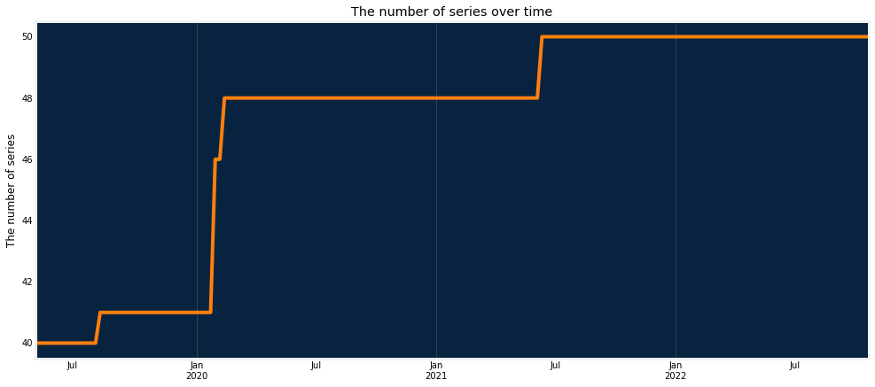
It is quite common for demand forecasting use cases to have series which don’t have sales any more, had temporary or seasonal sales, or were just released. The plot below shows how the number of series evolved over time for the chosen dataset.

In [17]:

dru.plot_series_count_over_time(df, date_col, series_id)

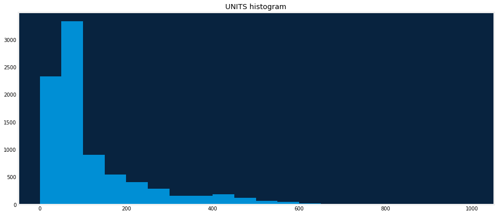
The target distribution plot can help to identify the most frequent values and the shape of data in general.

In [18]:

dru.plot_hist(df, target, clip_min=0)

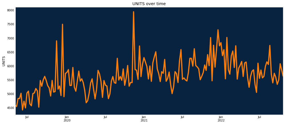
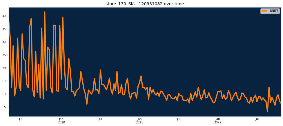
The plot of the target over time can show overall seasonality, trend, /or possible issues with the data (e.g., sudden drops or periods without data).

In [19]:

dru.plot_num_col_over_time(df, date_col, target, func="sum", freq="W-MON")

Data checks

Spikes

The dataset should be checked for anomalous spikes. They should be verified. If they are correct, they should be added to a calendar file, or some form of feature engineering should be completed so that the models can be able to predict these spikes.

In [20]:

df_spikes = dru.identify_spikes(df, date_col, series_id, target, span=5, threshold=7)
print(
    "# of series with spikes:", df_spikes[df_spikes["Spike"] == 1][series_id].nunique()
)
df_spikes[df_spikes["Spike"] == 1].sort_values(target, ascending=False).head()

# of series with spikes: 50

# of series with spikes: 50

Out[20]:

	STORE_SKU	DATE	UNITS	EWA	SD	Threshold	Spike
4770	store_175_SKU_120939350	2021-08-23	657.0	596.806961	85.265846	596.860920	1
4772	store_175_SKU_120939350	2021-09-06	649.0	597.580871	76.941499	538.590492	1
4769	store_175_SKU_120939350	2021-08-16	641.0	566.710441	86.652437	606.567057	1
4782	store_175_SKU_120939350	2021-11-15	634.0	570.983367	62.093165	434.652155	1
5391	store_175_SKU_9888909	2019-08-05	628.0	541.622103	76.445072	535.115503	1

In [21]:

sid = (
    df_spikes[df_spikes["Spike"] == 1]
    .sort_values(target, ascending=False)[series_id]
    .values.tolist()[0]
)
dru.plot_series_over_time(df_spikes, date_col, series_id, sid, [target, "EWA"])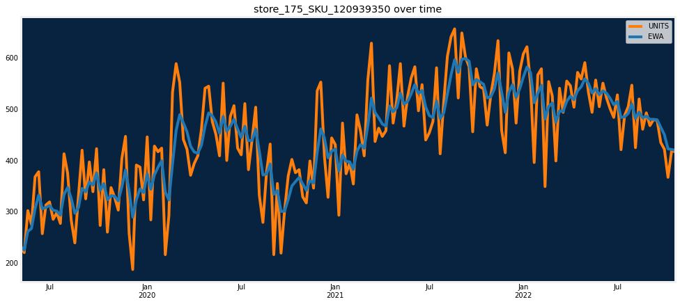

Negative values

Negative values should be also checked if they are correct.

In [22]:

series_neg = df_stats[df_stats["negatives"] > 0][series_id].unique().tolist()
print("# of series with negative values:", len(series_neg))
if len(series_neg) > 0:
    dru.plot_series_over_time(df, date_col, series_id, series_neg[0], [target])

# of series with negative values: 0

Duplicate datetimes

Duplicate datetimes within single series could be introduced by mistake.

In [23]:

series_dupl_dates = df.groupby([series_id, date_col])[date_col].count()
series_dupl_dates = series_dupl_dates[series_dupl_dates > 1]
print("# of series with duplicate dates:", len(series_dupl_dates))
if len(series_dupl_dates):
    print("eries with duplicate examples:", len(series_dupl_dates))
    print(series_dupl_dates.head())

# of series with duplicate dates: 0

Series start and end dates

Check if any series start after the the minimum datetime and if any series end before the maximum datetime.

In [24]:

series_new = (
    df_stats[df_stats["date_col_min"] > df_stats["date_col_min"].min()][series_id]
    .unique()
    .tolist()
)
series_old = (
    df_stats[df_stats["date_col_max"] < df_stats["date_col_min"].max()][series_id]
    .unique()
    .tolist()
)
print("# of new series:", len(series_new))
print("# of old series:", len(series_old))

# of new series: 10
# of old series: 0

Gaps

Completely missing records within the series should be verified.

In [25]:

df_stats.sort_values("gap_max", ascending=False).head()

Out [25]:

	0	37	27	28	29
STORE_SKU	store_130_SKU_120931082	store_192_SKU_909893792	store_175_SKU_120949681	store_175_SKU_120969012	store_175_SKU_409929345
rows	182	182	182	182	182
date_col_min	2019-05-06	2019-05-06	2019-05-06	2019-05-06	2019-05-06
date_col_max	2022-10-24	2022-10-24	2022-10-24	2022-10-24	2022-10-24
target_mean	127.401099	74.543956	395.049451	237.461538	75.258242
nunique	95	87	136	136	96
missing	0	0	0	0	0
zeros	0	0	0	0	1
negatives	0	0	0	0	0
gap_max	7 days	7 days	7 days	7 days	7 days
gap_mode	7 days	7 days	7 days	7 days	7 days
gap_uncommon_count	0	0	0	0	0
duration	1268	1268	1268	1268	1268
rows_to_duration	0.143533	0.143533	0.143533	0.143533	0.143533
missing_rate	0	0	0	0	0
zeros_rate	0	0	0	0	0.005495

In [26]:

dru.plot_series_over_time(
    df,
    date_col,
    series_id,
    df_stats.sort_values("gap_max", ascending=False)[series_id].values[0],
    [target],
)

Modeling

The next step after the data preparation and before modeling is to specify the modeling parameters:

• Features known in advance are things you know in the future, such as product metadata or a planned marketing event. If all features are known in advance, use the setting default_to_known_in_advance.
• Do not derive features will be excluded from deriving time-related features. If all features should be excluded, default_to_do_not_derive can be used.
• metric is used for evaluating models. DataRobot supports a wide variety of metrics. The metric used depends on the use case. If the value is not specified, DataRobot suggests a metric based on the target distribution.
• feature_derivation_window_start and feature_derivation_window_end define the feature derivation window (FDW). The FDW represents the rolling window that is used to derive time series features and lags. FDW definition should be long enough to capture relevant trends to your use case. On the other hand, FDW shouldn’t be too long (e.g., 365 days) because it shrinks the available training data and increases the size of the feature list. Older data does not help the model learn recent trends. It is not necessary to have a year-long FDW to capture seasonality; DataRobot auto-derives features (month indicator, day indicator), as well as learns effects near calendar events (if a calendar is provided), in addition to blueprint specific techniques for seasonality.
• gap_duration is the duration of the gap between training and validation/holdout scoring data, representing delays in data availability. For example, at prediction time, if events occuring on Monday aren’t reported or made available until Wednesday, you would have a gap of 2 days. This can occur with reporting lags or with data that requires some form of validation before being stored on a system of record.
• forecast_window_start and forecast_window_end defines the forecast window (FW). It represents the rolling window of future values to predict. FW depends on a business application of the model predictions.
• number_of_backtests and validation_duration. Proper backtest configuration helps evaluate the model’s ability to generalize to the appropriate time periods. The main considerations during the backtests specification are listed below.
  • Validation from all backtests combined should span the region of interest.
  • Fewer backtests means the validation lengths might need to be longer.
  • After the specification of the appropriate validation length, the number of backtests should be adjusted until they span a full region of interest.
  • The validation duration should be at least as long as your best estimate of the amount of time the model will be in production without retraining.
• holdout_start_date with one of holdout_end_date or holdout_duration can be added additionally. DataRobot will define them based on validation_duration if they were not specified.
• calendar_id is the ID of the previously created calendar. DataRobot automatically create features based on the calendar events (such as “days to next event” ). There are several options to create a calendar:
  • From an AI Catalog dataset:calendar = dr.CalendarFile.create_calendar_from_dataset(dataset_id)
  • Based on the provided country code and dataset start date and end dates:calendar = dr.CalendarFile.create_calendar_from_country_code(country_code, start_date, end_date)
  • From a local file:calendar = dr.CalendarFile.create(path_to_calendar_file)
• allow_partial_history_time_series_predictions – Not all blueprints are designed to predict on new series with only partial history, as it can lead to suboptimal predictions. This is because for those blueprints the full history is needed to derive the features for specific forecast points. “Cold start” is the ability to model on series that were not seen in the training data; partial history refers to prediction datasets with series history that is only partially known (historical rows are partially available within the feature derivation window). If True, Autopilot will run the blueprints optimized for cold start and also for partial history modeling, eliminating models with less accurate results for partial history support.
• segmented_project set to True and the cluster name cluster_id can be used for segmented modeling. This feature offers the ability to build multiple forecasting models simultaneously. DataRobot creates multiple projects “under the hood”. Each project is specific to its own data per cluster_id. The model benefits by having forecasts tailored to the specific data subset, rather than assuming that the important features are going to be the same across all of series. The models for different cluster_ids will have features engineered specifically from cluster-specific data. The benefits of segmented modeling also extend to deployments. Rather than deploying each model separately, we can deploy all of them at once within one segmented deployment.

The function dr.helpers.partitioning_methods.construct_duration_string() can be used to construct a valid string representing the gap_duration, validation_duration and holdout_duration duration in accordance with ISO8601.

Create a calendar

Create a calendar based on the dataset in the AI Catalog.

In [ ]:

calendar = dr.CalendarFile.create_calendar_from_dataset(
    dataset_id=dataset_calendar.id, calendar_name=dataset_calendar.name
)
calendar_id = calendar.id

Configure modeling settings

In [ ]:

features_known_in_advance = ["STORE", "SKU", "SKU_CATEGORY", "PROMO_MAX"]
do_not_derive_features = ["STORE", "SKU", "SKU_CATEGORY"]

params = {
    "metric": None,
    "features_known_in_advance": features_known_in_advance,
    "do_not_derive_features": do_not_derive_features,
    "target": target,
    "mode": "quick",
    "segmented_project": False,
    "cluster_id": None,
    "datetime_partition_column": date_col,
    "multiseries_id_columns": [series_id],
    "use_time_series": True,
    "feature_derivation_window_start": None,
    "feature_derivation_window_end": None,
    "gap_duration": None,
    "forecast_window_start": None,
    "forecast_window_end": None,
    "number_of_backtests": None,
    "validation_duration": None,
    "calendar_id": calendar_id,
    "allow_partial_history_time_series_predictions": True,
}

Create and run projects

Run projects using the function dru.run_projects and wait for completion. The arguments:

• data – a dr.Dataset, a pandas DataFrame or a path to a local file
• params – a dictionary with parameters as specified in the description and example above. return a nested dictionary of {project.id: {project meta-data : values,...}}. Defaults to one project unless segmented modeling is enabled

In [29]:

projects = dru.run_projects(
    data=dataset_train,
    params=params,
    description="all series",
    file_to_save="projects_test.csv",
)

DataRobot will define FDW and FD automatically.
2023-01-20 18:03:33.759359 start: UNITS_20230120_1803

In [44]:

projects

Out [44]:

{'63cb1dc57f7acc3548033664': {'project': Project(UNITS_20230120_1803),
  'project_name': 'UNITS_20230120_1803',
  'project_type': 'all series',
  'cluster_id': None,
  'cluster_name': None,
  'description': 'all series',
  'deployment_id': '63cb208ca24ba50de23d8825',
  'deployment': Deployment(UNITS_20230120_1803),
  'preds_job_def': BatchPredictionJobDefinition(63cb20f6a015dc87b07d1637),
  'preds_job_def_id': '63cb20f6a015dc87b07d1637'}}

Initiate Autopilot

In [30]:

for cl, vals in projects.items():
    proj = vals["project"]  # DataRobot Project Object
    print(proj.id, proj)
    proj.wait_for_autopilot(verbosity=dr.enums.VERBOSITY_LEVEL.SILENT)

63cb1dc57f7acc3548033664 Project(UNITS_20230120_1803)

Model evaluation and insights

Select a project to take a closer look at model performance.

In [31]:

project = list(projects.values())[0]["project"]
if project.is_segmented:
    combined_model = project.get_combined_models()[0]
    segments_df = combined_model.get_segments_as_dataframe()
    project = dr.Project.get(
        segments_df.sort_values("row_percentage", ascending=False)["project_id"][0]
    )

print(project.id, project)

63cb1dc57f7acc3548033664 Project(UNITS_20230120_1803)

Retrieve models

Select the most accurate model from the Leaderboard.

In [32]:

model_scores = dru.get_leaderboard(project)
model = model_scores["model"][0]
print(model.id, model)
model_scores.head()

63cb1e6e40ff7079faba3407 DatetimeModel('eXtreme Gradient Boosting Regressor with Early Stopping and New Series Support')

	0	1	2	3	4
project_id	63cb1dc57f7acc3548033664	63cb1dc57f7acc3548033664	63cb1dc57f7acc3548033664	63cb1dc57f7acc3548033664	63cb1dc57f7acc3548033664
blueprint_id	10807011a661cff2077ffcae75a240f5	10807011a661cff2077ffcae75a240f5	919fd7caa918c51626dcdcbf3e4a2fe5	f7b1dd1f2967237ac8aec1510e1a2c48	586e48c7da793c3384aa5102caaef2e5
featurelist_id	63cb1e317157b7ddd0784314	63cb1f40eb25b482359d0195	63cb1e317157b7ddd0784314	63cb1e317157b7ddd0784314	63cb1e317157b7ddd0784314
model_id	63cb1e6e40ff7079faba3407	63cb1f41eb25b482359d019c	63cb1e6e40ff7079faba3406	63cb1e6e40ff7079faba3403	63cb1e6e40ff7079faba3404
model_n	15	36	14	11	12
model_cat	model	model	model	model	model
model_type	eXtreme Gradient Boosting Regressor with Early…	eXtreme Gradient Boosting Regressor with Early…	eXtreme Gradient Boosting Regressor with Early…	Performance Clustered eXtreme Gradient Boosted…	Temporal Hierarchical Model with Elastic Net a…
model	DatetimeModel(‘eXtreme Gradient Boosting Regre…	DatetimeModel(‘eXtreme Gradient Boosting Regre…	DatetimeModel(‘eXtreme Gradient Boosting Regre…	DatetimeModel(‘Performance Clustered eXtreme G…	DatetimeModel(‘Temporal Hierarchical Model wit…
duration	P0Y0M797D	P0Y0M797D	P0Y0M797D	P0Y0M797D	P0Y0M797D
end_date	NaT	NaT	NaT	NaT	NaT
RMSE_backtests	43.79093	43.82645	44.04191	44.92713	45.56763
RMSE_backtest1	34.57502	34.24454	32.926	34.66657	34.62065

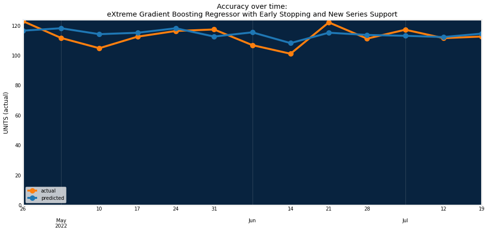
Accuracy over time

Accuracy over time helps visualize how predictions change over time compared to actuals.

In [33]: 

dru.plot_accuracy_over_time(project, model)

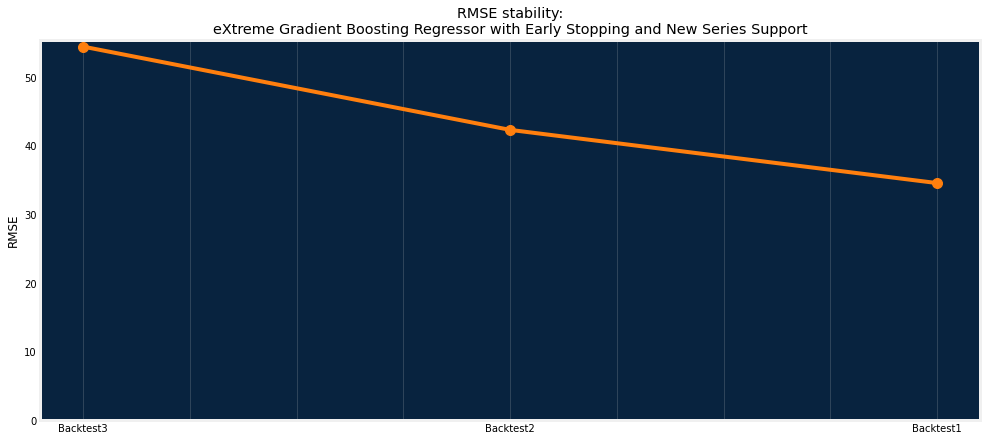
Stability

View an at-a-glance summary of how well a model performs on different backtests.

In [34]:

dru.plot_stability_scores(project, model)

Series insights

Series insights provide data representing accuracy, average scores, length, and start/end date distribution by count for each series.

In [35]:

model_sa = dru.get_series_accuracy(project, model, compute_all_series=True)
print("project metric:", project.metric)
print(model_sa.shape)
model_sa.head()

project metric: RMSE
(50, 10)

	0	1	2	3	4
multiseriesId	63cb1df7f8f3aac9f4cba3ce	63cb1df7f8f3aac9f4cba3cf	63cb1df7f8f3aac9f4cba3d0	63cb1df7f8f3aac9f4cba3d1	63cb1df7f8f3aac9f4cba3d2
multiseriesValues	[store_130_SKU_120931082]	[store_130_SKU_120969795]	[store_133_SKU_9888998]	[store_136_SKU_120973845]	[store_137_SKU_120949681]
rowCount	182	182	182	182	182
duration	P3Y5M18D	P3Y5M18D	P3Y5M18D	P3Y5M18D	P3Y5M18D
startDate	2019-05-06T00:00:00.000000Z	2019-05-06T00:00:00.000000Z	2019-05-06T00:00:00.000000Z	2019-05-06T00:00:00.000000Z	2019-05-06T00:00:00.000000Z
endDate	2022-10-24T00:00:00.000000Z	2022-10-24T00:00:00.000000Z	2022-10-24T00:00:00.000000Z	2022-10-24T00:00:00.000000Z	2022-10-24T00:00:00.000000Z
validationScore	11.47039	17.91493	19.46449	18.622	30.88644
backtestingScore	17.603	21.46553	14.69731	20.04677	105.254205
holdoutScore	22.04872	21.05725	22.61437	23.13299	62.46387
targetAverage	127.401099	46.098901	46.986264	88.274725	232.565934

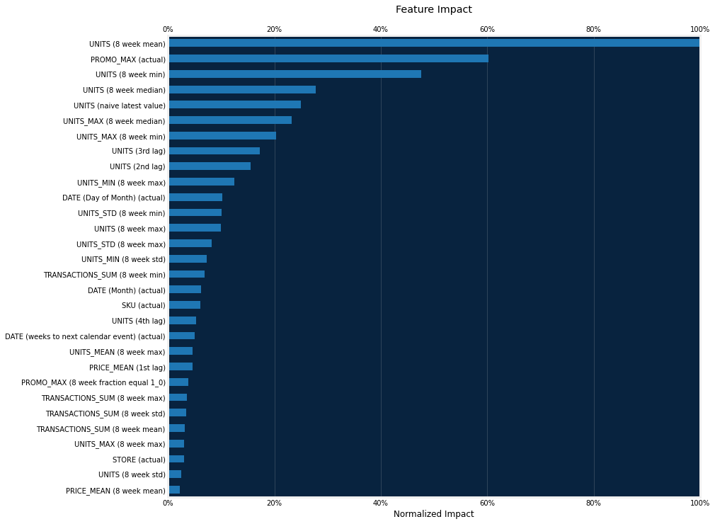
Feature Impact

Feature Impact is available for all model types and works by altering input data and observing the effect on a model’s score. It is an on-demand feature, meaning that you must initiate a calculation to see the results. Once you have had DataRobot compute the feature impact for a model, that information is saved with the project.

Feature Impact measures how important a feature is in the context of a model. That is, it measures how much the accuracy of a model would decrease if that feature were removed.

Note that the diversity of features created is providing signal to the model.

In [36]:

dru.plot_feature_impacts(model, top_n=30)

Deployment

After you have selected your final model, you have multiple options for a production deployment in DataRobot MLOps. Creating a deployment will add your model package to the Model Registry and containerize all model artifacts, generate compliance documentation, expose a production quality REST API on a prediction server in your DataRobot cluster, and enable all lifecycle management fucntionality, like drift monitoring. Two helper function are provided below:

dru.make_deployments accepts a dictionary of projects and deploys the DataRobot recommended model. This will enable multiple deployments if you are using segmented modeling, which can be helpful if you have many segments (and thus many models to deploy).

dru.make_deployment can be used to deploy a specific model by passing the model.id. If model.id is None, the DataRobot recommended model from the project will be deployed.

In [37]:

deployments = dru.make_deployments(
    projects, file_to_save="deployments_test.csv", feature_drift_enabled=True
)

Deployment ID: 63cb208ca24ba50de23d8825; URL: https://app.datarobot.com/deployments/63cb208ca24ba50de23d8825/overview

In [46]:

dep2 = dru.make_deployment(
    project=project,
    name="Temporal Hierarchical Model with Elastic Net and XGBoost",
    model_id="63cb1e6e40ff7079faba3404",
)

Deployment ID: 63cb51522fe7840c4fa43cfd; URL: https://app.datarobot.com/deployments/63cb51522fe7840c4fa43cfd/overview

Make predictions

The scoring dataset should follow requirements to ensure the Batch Prediction API can make predictions:

• Sort prediction rows by their series ID then timestamp, with the earliest row first.
• The dataset must contain rows without a target for the desired forecast window.

You can find more details on the scoring dataset structure in the DataRobot documentation.

Batch predictions on demand

Select the data from your data store, make predictions, and write them back to Snowflake once processed.

In [38]:

intake_settings = {
    "type": "jdbc",
    "data_store_id": data_store_id,
    "credential_id": credential_id,
    "query": f'select * from {db}.{schema}."ts_demand_forecasting_scoring" order by {series_id}, {date_col};',
}

output_settings = {
    "type": "jdbc",
    "data_store_id": data_store_id,
    "credential_id": credential_id,
    "table": "ts_demand_forecasting_predictions",
    "schema": schema,
    "catalog": db,
    "create_table_if_not_exists": True,
    "statement_type": "insert",
}

pred_jobs = dru.make_predictions(
    deployments=deployments,
    intake_settings=intake_settings,
    output_settings=output_settings,
    passthrough_columns_set=None,
    passthrough_columns=["SKU", "STORE"],
)

2023-01-20 18:16:21.003062 start: UNITS_20230120_1803 predictions

Scheduled batch predictions

Use prediction job definitions to make batch predictions on a schedule.

In [39]:

intake_settings = {
    "type": "jdbc",
    "data_store_id": data_store_id,
    "credential_id": credential_id,
    "query": f'select * from {db}.{schema}."ts_demand_forecasting_scoring" order by {series_id}, {date_col};',
}

output_settings = {
    "type": "jdbc",
    "data_store_id": data_store_id,
    "credential_id": credential_id,
    "table": "ts_demand_forecasting_predictions",
    "schema": schema,
    "catalog": db,
    "create_table_if_not_exists": True,
    "statement_type": "insert",
}

schedule = {
    "minute": [0],
    "hour": [23],
    "day_of_week": ["*"],
    "day_of_month": ["*"],
    "month": ["*"],
}

deployments = dru.create_preds_job_definitions(
    deployments=deployments,
    intake_settings=intake_settings,
    output_settings=output_settings,
    enabled=False,
    schedule=schedule,
    passthrough_columns_set=None,
    passthrough_columns=["SKU", "STORE"],
)

2023-01-20 18:17:09.453436 start: UNITS_20230120_1803 create predictions job definition

In [40]:

# # Run predictions job definitions manually

# for pid, vals in deployments.items():
#     vals['preds_job_def'].run_once()

Get predictions

In the previous step, you ran prediction jobs from your registered data store (Snowflake) with your prediciton dataset, ts_demand_forecasting_scoring . The steps below add the new prediction table, ts_demand_forecasting_predictions, to the AI Catalog. This enables versioning of each prediciton run, and completing the governance loop for traceability from scoring data to model to predicition data.

In [41]:

# Create or get an existing data connection based on a query and upload the predictions into AI Catalog

data_source_preds, dataset_preds = dru.create_dataset_from_data_source(
    data_source_name="ts_preds_data",
    query=f'select * from {db}.{schema}."ts_demand_forecasting_predictions";',
    data_store_id=data_store_id,
    credential_id=credential_id,
)

new data source: DataSource('ts_preds_data')

The table with predictions has the following schema:

• {SERIES_ID_COLUMN_NAME} is the series ID the row belongs to. In this demo the column name is STORE_SKU.
• FORECAST_POINT is the timestamp ou are making a prediction from.
• {TIME_COLUMN_NAME} is the time series timestamp the predictions were made for. In this demo the column name is DATE.
• FORECAST_DISTANCE is a unique relative position within the Forecast Window. A model outputs one row for each Forecast Distance.
• <target_name>_PREDICTION
• DEPLOYMENT_APPROVAL_STATUS. If the approval workflow is enabled for the deployment, the output schema will contain an extra column showing the deployment approval status.
• Other columns specified in passthrough_columns or all columns from the prediction dataset if passthrough_columns_set='all'.

You can find more details on the predictions structure in the DataRobot documentation.

In [42]:

# Get predictions as a dataframe

df_preds = dataset_preds.get_as_dataframe()
df_preds[date_col] = pd.to_datetime(df_preds[date_col], format="%Y-%m-%d")
df_preds.sort_values([series_id, date_col], inplace=True)
print("the original data shape   :", df_preds.shape)
print("the total number of series:", df_preds[series_id].nunique())
print("the min date:", df_preds[date_col].min())
print("the max date:", df_preds[date_col].max())
df_preds.head()

the original data shape   : (200, 8)
the total number of series: 50
the min date: 2022-10-30 17:00:00
the max date: 2022-11-20 16:00:00

	0	199	198	197	196
STORE_SKU	store_130_SKU_120931082	store_130_SKU_120931082	store_130_SKU_120931082	store_130_SKU_120931082	store_130_SKU_120969795
FORECAST_POINT	2022-10-23 17:00:00	2022-10-23 17:00:00	2022-10-23 17:00:00	2022-10-23 17:00:00	2022-10-23 17:00:00
DATE	2022-10-30 17:00:00	2022-11-06 16:00:00	2022-11-13 16:00:00	2022-11-20 16:00:00	2022-10-30 17:00:00
FORECAST_DISTANCE	1	2	3	4	1
UNITS (actual)_PREDICTION	77.779026	78.455166	80.292369	89.63322	66.912723
DEPLOYMENT_APPROVAL_STATUS	APPROVED	APPROVED	APPROVED	APPROVED	APPROVED
SKU	SKU_120931082	SKU_120931082	SKU_120931082	SKU_120931082	SKU_120969795
STORE	store_130	store_130	store_130	store_130	store_130

Conclusion

This notebook’s workflow provides a repeatable framework from project setup to model deployment for times series data with multiple series (SKUs) with full, partial and no history. This notebook presented frameworks for aggregation at the SKU and store-SKU level, and provided functions to streamline building and deploying multiple models from time series projects with and without Segmented Modeling enabled. It also provided helpers to extract series and model insights for common challenges seen in real-world data, and multiple methods for prediciton and production deployment with full MLOps capabilities. The steps above provide many of the building blocks necessary for evaluating and experimenting on complex, real-world multi-series data.

An extremely common practice in the field is running experiments with various feature derivation windows and forecast distances. For example, if a business desires predictions 6 months out, and you have a few years of history, the best model to predict 3-6 months out may not be the same model that best predicts 1-3 months out. Conceptually, recall that DataRobot generates a wide range of lagged features based on the Feature Derivation Window. The features that best capture short-term predictions (with customer data, this can be lags of a few days or weeks and product interactions), can quite reasonably not be the same set of features that capture mid to long-term predictions. This can be compounded when you have a large number of series/SKUs; many blueprints are designed to learn interactions and trends across series, which again can have different interaction effects and periodicities. This is usually a good indicator to use Segmented Modeling. At the same time, one model could work quite well depending on the dynamics of your target. There is no silver bullet, hence the benefit of learning how to apply automation to rapidly experiment and improve your models.

In all cases, ensuring your validation period captures the behavior you want to predict, and that your backtests do as well, is vitally important.

Try experimenting with differnet Forecast Distances and compare the important features across projects. Enable the various project settings in the params dictionary in the Run Projects section, and enable Segmented Modeling. Identify and evaluate the peformance of some of the partial history series. Getting comfortable with these common workflows will accelerate your time to value in future projects.

Delete project artifacts

Optional.

In [43]:

# # Uncomment and run this cell to remove everything you added in DataRobot during this session

# dr.Dataset.delete(dataset_train.id)
# dr.Dataset.delete(dataset_calendar.id)
# dr.Dataset.delete(dataset_preds.id)

# data_source_train.delete()
# data_source_calendar.delete()
# data_source_preds.delete()

# _ = [d['preds_job_def'].delete() for d in list(deployments.values())]

# _ = [d['deployment'].delete() for d in list(deployments.values())]

# _ = [p['project'].delete() for p in list(projects.values())]

# dr.CalendarFile.delete(calendar_id)