Understanding Models in DataRobot. Overview

This post was originally part of the DataRobot Community. Visit now to browse discussions and ask questions about the DataRobot AI Platform, data science, and more.

DataRobot offers many Explainable AI tools to help you understand your models. Three model-agnostic approaches can be found in the Understand tab: Feature Impact, Feature Effects, and Prediction Explanations. This article covers these methods as well as Word Cloud which is useful in models with text data.

Feature Impact

Feature Impact can be found on the Understand > Feature Impact tab of the model that you are interested in. 

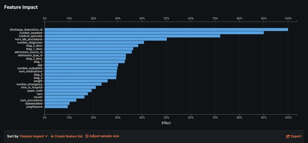
Feature Impact is a model-agnostic approach that informs us of the most important features of our model. The methodology used to calculate this impact is called permutation importance. This calculation normalizes the results so that the most important feature will always have a feature impact score of 100%, and the other features Impact scores will be set relative to that. 

If you want to aim for parsimonious models, you can remove features with low feature impact scores. To do this, create a new feature list (in the Feature Impact tab) that has the top features and build a new model for that feature list. You can then compare the difference in model performance and decide whether the parsimonious model is better for your use case.

Furthermore, even though it is not that common, features can also have a negative feature impact score. When this is the case, it will appear as if the features are not improving model performance. You may consider removing them and evaluating the effect on model performance.

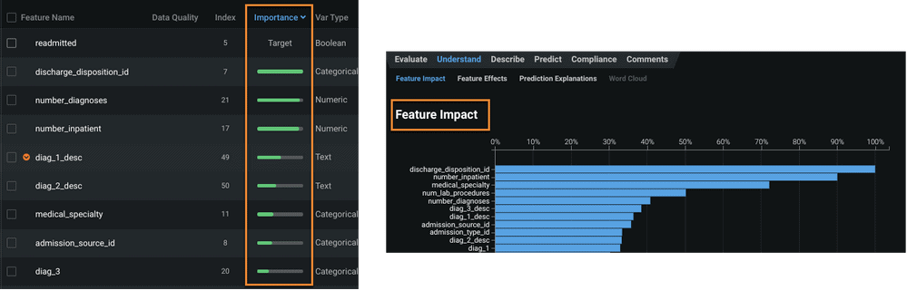
Lastly, be aware that feature impact differs from the importance measure shown in the Data page. The green bars displayed in the Importance column of the Data page are a measure of how much a feature, by itself, is correlated with the target variable. By contrast, Feature Impact measures how important a feature is in the context of a model. In other words, Feature Impact measures how much (based on the training data) the accuracy of a model would decrease if that feature were removed.

Feature Effects

Feature Effects identifies how a feature impacts the overall predictive capability of the model. This is achieved using another model-agnostic approach called partial dependence.  

In the image below we have an example using the num_inpatient visits from our Readmission example. You can see that as the number of inpatient visits increases, the likelihood of readmission increases in kind. This helps you understand why your features are predictive and can give you deep insights into the patterns of your data.  

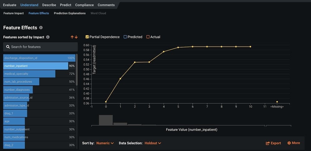
The partial dependence shown in Figure 4 illustrates that the marginal effect (or “holding everything else constant”) effect of inpatient is to raise the probability of readmission from 0.36 at 0 to a maximum around 0.60 when number_inpatient is 6.  

Prediction Explanations

Feature Impact and Feature Effects give you global insight into how your features are impacting your predictions. Prediction Explanations give you local insight into how your features are impacting your predictions on a row-by-row basis. 

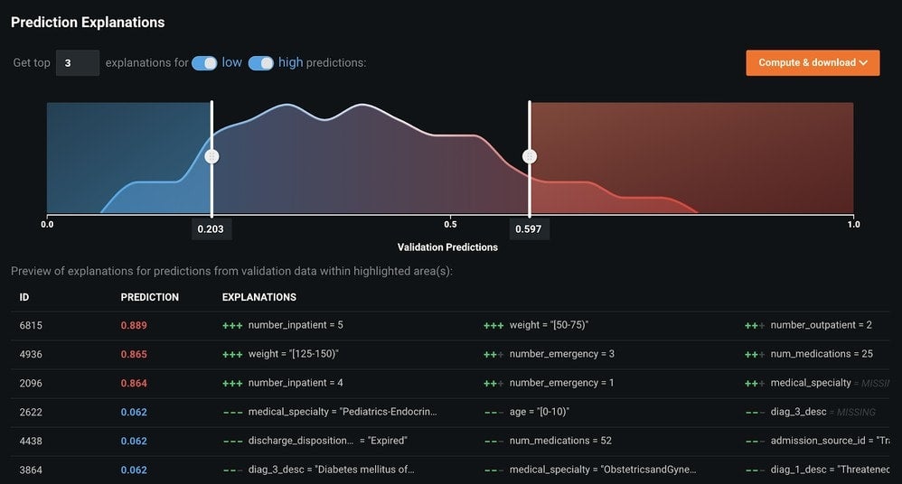
If you select Understand > Prediction Explanations you will see a summary of the Prediction Explanations. The page shows a sample of three rows from the high end and three rows from the low end of the prediction distribution; however, you can compute and download explanations for every row in your dataset. You can get up to 10 Prediction Explanations per row (in our example, each row is a loan application).

Figure 5 shows the predictions indicated in red or blue text. The red predictions are at the high-end of the prediction distribution (i.e., close to 1), while the blue predictions are on the low-end distribution (i.e., close to 0).  The +++ and — indicate the strength and direction of the relationship. In the first row, number_inpatient is quite high and is strongly pushing the prediction probability up (+++). In the last row, the feature discharge_disposition is “Expired” and pushing the prediction probability down (—). In the case of this feature, the Prediction Explanations have revealed a potential issue with our data. If a patient is deceased, then of course they are not going to be readmitted to the hospital.  

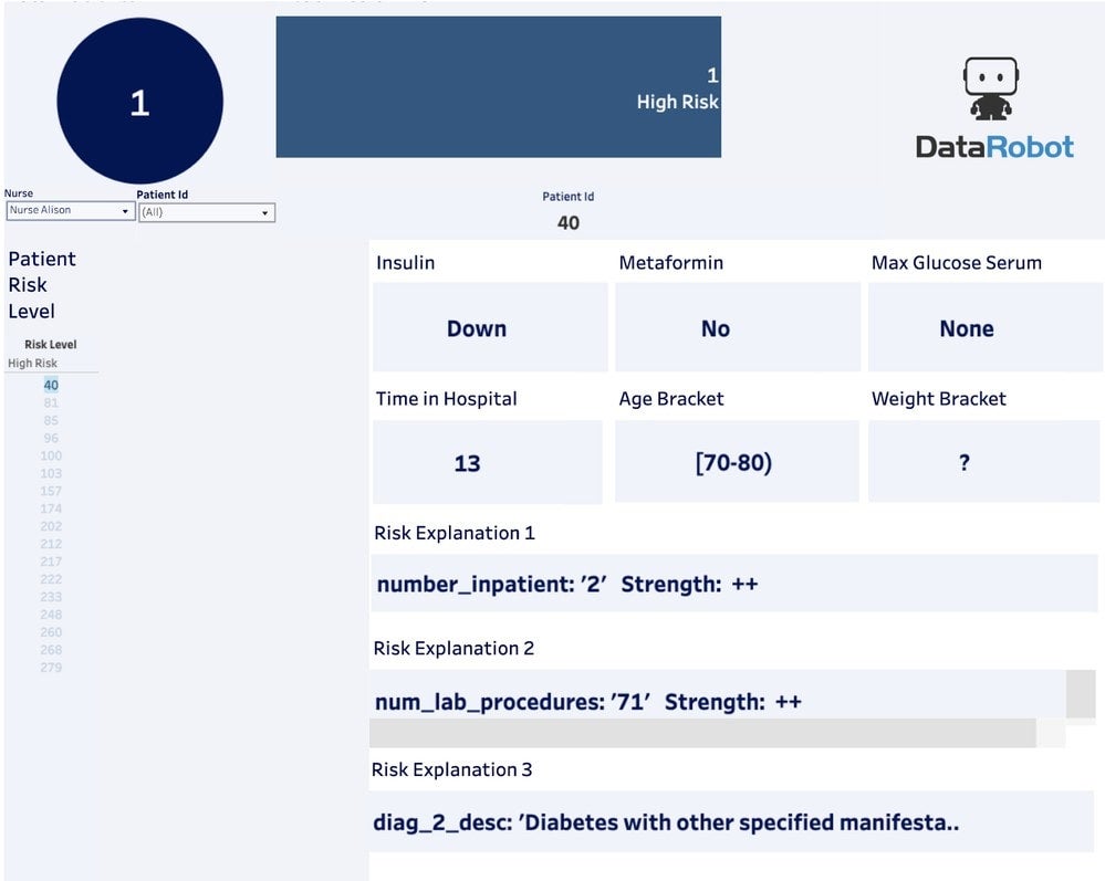
Prediction Explanations are especially useful for communicating results with non-data scientists. For example, if you have a nurse that doesn’t know anything about machine learning, you can show Prediction Explanations and they will understand why the features are making the patients high or low risk. This is important because, in our use case, the nurse is the end user and needs to be able to easily interpret Prediction Explanations. The modeling scores are going to impact this person’s day-to-day decision making.  Prediction Explanations allow them to leverage their domain expertise with the modeling results. Below you can see a dashboard that highlights how to potentially use these in BI Software.

Word Cloud

You can find the Word Cloud under the Insights tab. 

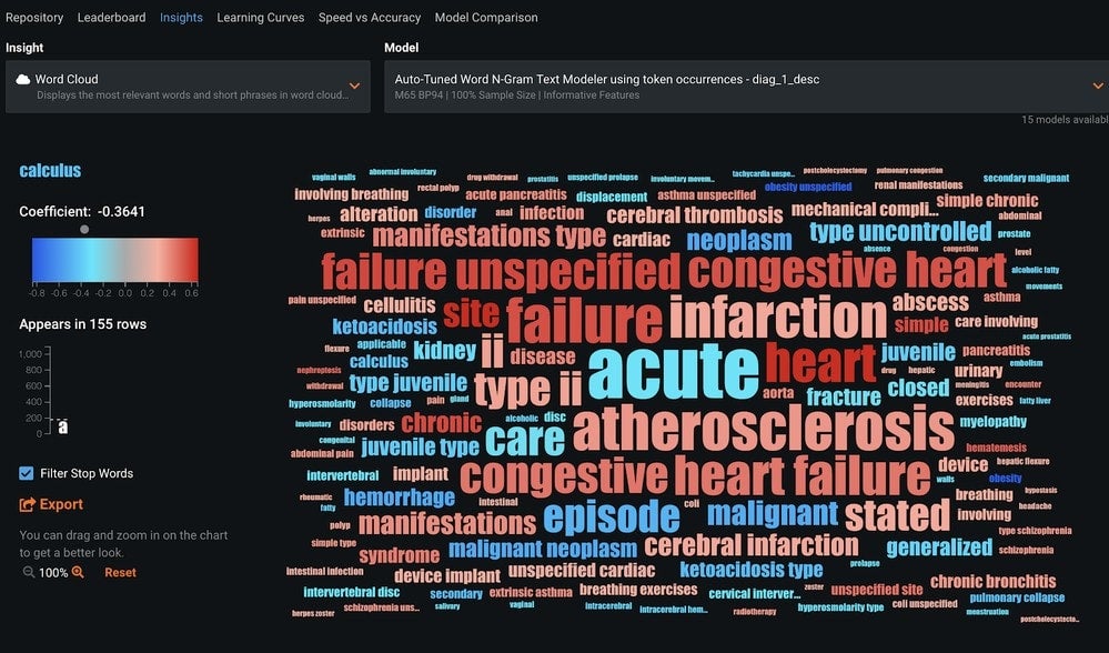
When you select Word Cloud you will see a visualization of the text features and their relationship to the target. This image is the result of an NLP Autotuned Word n-Gram Text model that used a preprocessing step in the model you are evaluating. 

The size of a word indicates its frequency in the dataset, where larger words appear more frequently than smaller ones.

The color indicates how it’s related to the target: 

• Words closer to the red end of the spectrum are associated with a higher target value, such as a 1 vs 0 in a binary classification problem, or a larger numeric value in a regression problem. 
• Words closer to the blue end of the spectrum are associated with a lower target value, such as a 0 vs 1 in a binary classification problem, or a lower numeric value in a regression problem. 

For example, in Figure 8 you can see that “heart” is more closely related to the target (diag_1_desc) than “acute.”

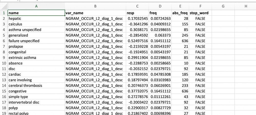
You can click the Export button to export the word cloud as an image or as a CSV file that contains the raw values. The exported CSV gives you a number of useful fields for each text feature in your dataset, including the word, the feature name, the strength of the correlation, and the frequency as a proportion of the total words and absolute measure. 

More Information

Search the DataRobot Platform Documentation for Feature Impact, Feature Effects, Prediction Explanations, and Word Cloud.

About the author

Linda Haviland

Community Manager

Meet Linda Haviland