Solving regression problem: NBA Player Performance

This post was originally part of the DataRobot Community. Visit now to browse discussions and ask questions about the DataRobot AI Platform, data science, and more.

This article summarizes how to solve a regression problem with DataRobot. Specifically, the topics include importing data, exploratory data analysis, and target selection, as well as modeling options, evaluation, interpretation and deployment.

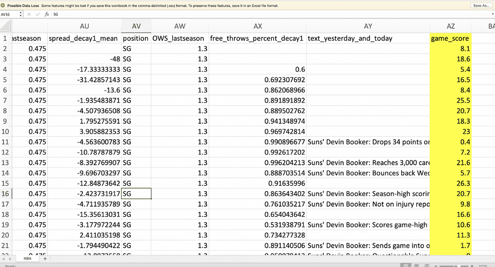
For this example we are using a historical dataset from NBA games. This is a sports dataset. Within it is a combination of raw and engineered features in various sources. We’re going to use this dataset to predict game_score, which is an advanced single statistic that attempts to quantify basketball player performance and productivity.

The different rows represent different basketball players within this dataset and the columns represent features about those players. At the end of this dataset, we have our target column indicated in yellow: this is the outcome that we’re trying to predict. The target here is a continuous variable, which makes this machine learning problem a ‘regression’ problem.

Importing Data

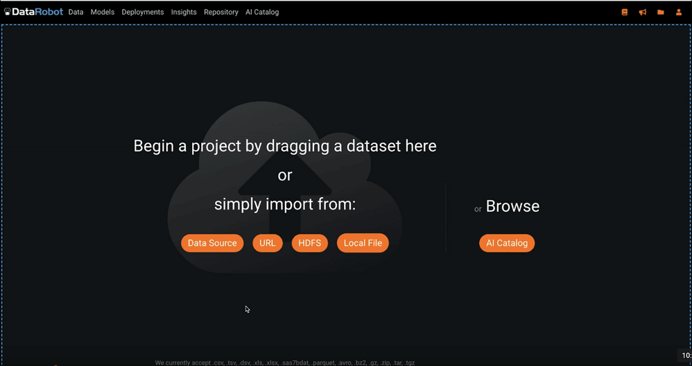
There are five ways to get data into DataRobot:

• Import data via a database connection using Data Source.
• Use a URL, such as an Amazon S3 bucket using URL.
• Connect to Hadoop using HDFS.
• Upload a local file using Local File.
• Create a project from the AI Catalog.

Exploratory Data Analysis

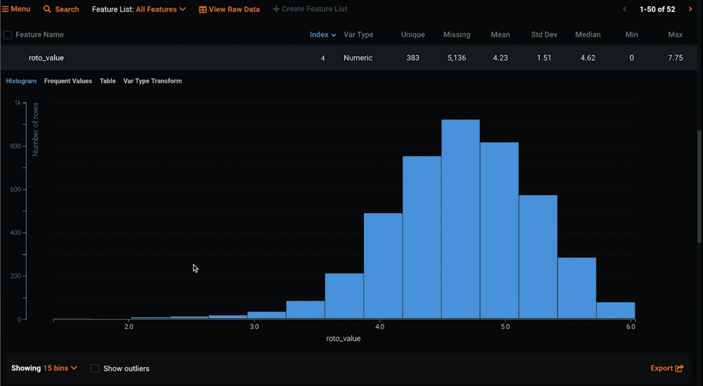
After you import your data, DataRobot will do an exploratory data analysis (EDA). This gives you the means, medians, unique, and missing values for each feature in your dataset.

If you want to look at a feature in more detail, simply click on it and a distribution will drop down.

Target Selection

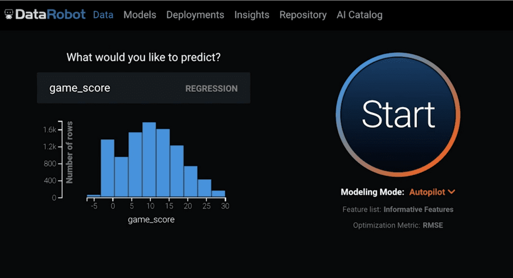
When you are done exploring your features, it is time to tell DataRobot the target feature (i.e., basketball game_score). You do this simply by scrolling up and entering it into the text field (as indicated in Figure 4). DataRobot will identify the problem type and give you a distribution of the target.

Modeling Options

At this point, you could simply hit the Start button to run Autopilot; however, there are some defaults that you can customize before building models.

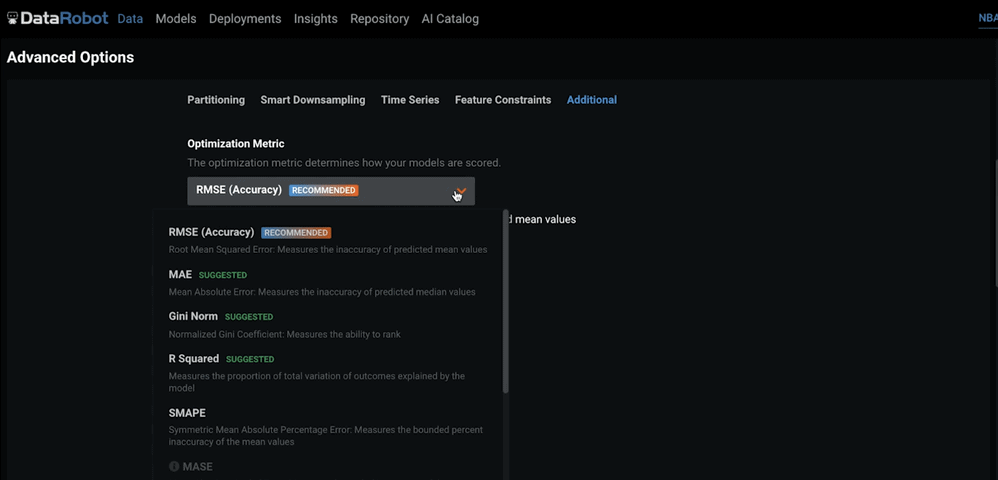
For example, under Advanced Options > Advanced, you can change the optimization metric:

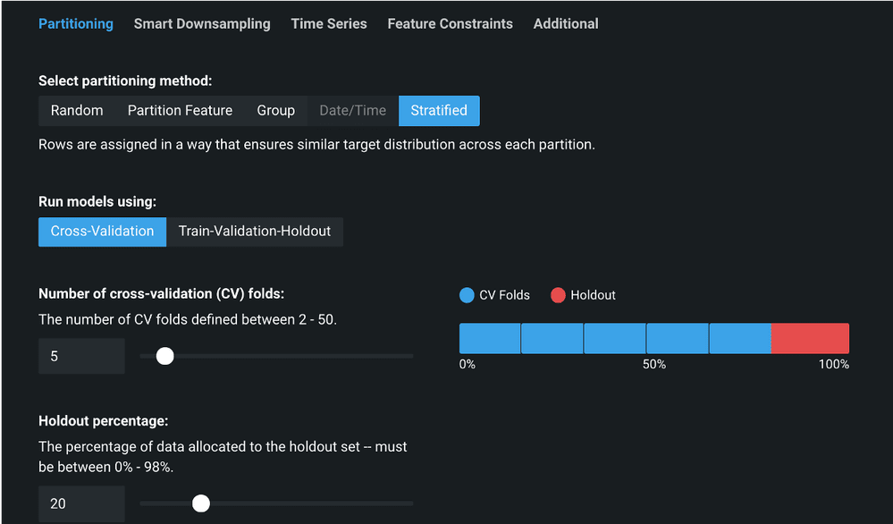
Then also, under Partitioning, you can also change the default partitioning:

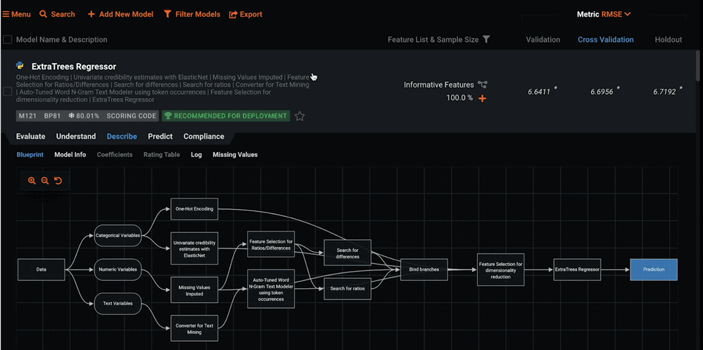
Once you are happy with the modeling options and have pressed Start, DataRobot creates 30–40 models; it does this through a process of building something called blueprints (see Figure 7). Blueprints are a set of preprocessing steps and modeling techniques specifically assembled to best fit the shape and distribution of your data. Every model that the platform creates contains a blueprint.

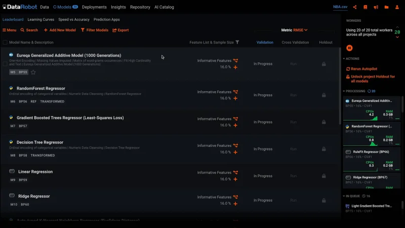
Model Evaluation

The models that DataRobot created will be ranked on the Leaderboard (see Figure 8). You can find this under the Models tab.

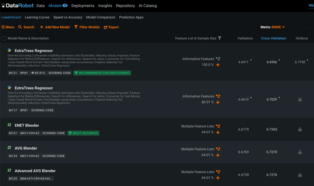
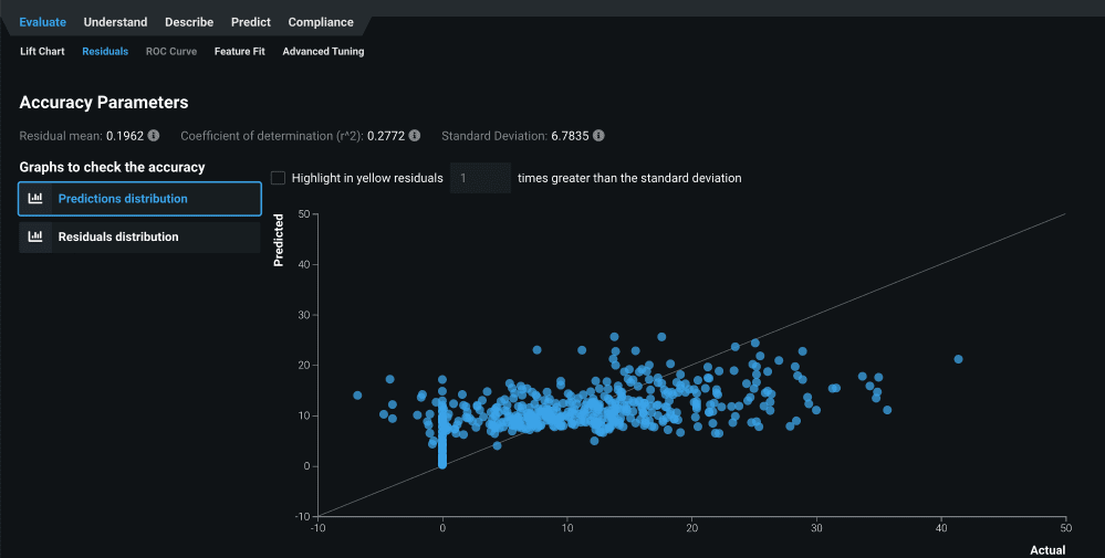
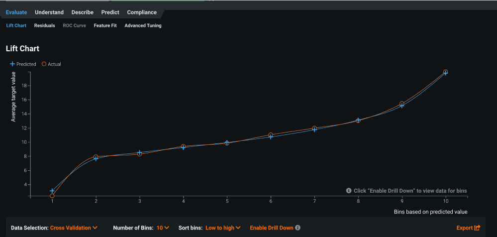
After you select a model from the Leaderboard and examine the blueprint, the next step is to evaluate the model. You can find a set of the evaluation metrics typically used in data science under Evaluate > Residuals (Figure 9a) and Evaluate > Lift (Figure 9b).

In the Residual chart you can see predicted and actual values.

In the Lift chart you can see how well the model fits across the prediction distribution.

Model Interpretation

Once you have evaluated your model for fit, it is time to take a look at how the different features are affecting predictions. You can find a set of interpretability tools in the Understand division.

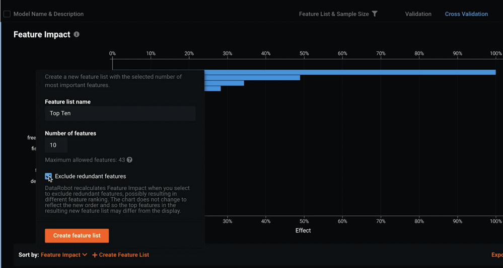
Feature Impact allows you to see which features are most important to your modeling.

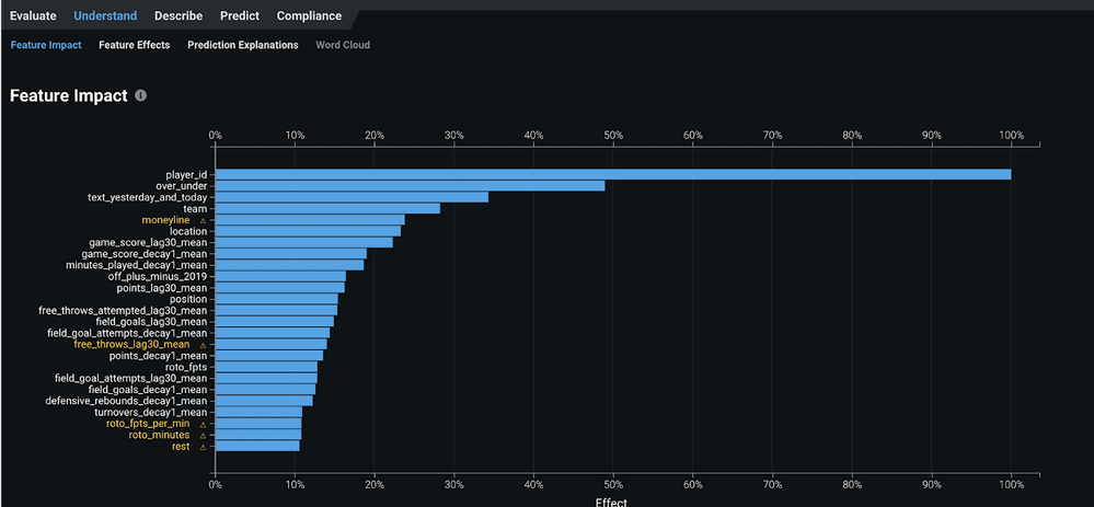
This is calculated using model-agnostic approaches. You can do a feature impact analysis for every model that DataRobot creates.

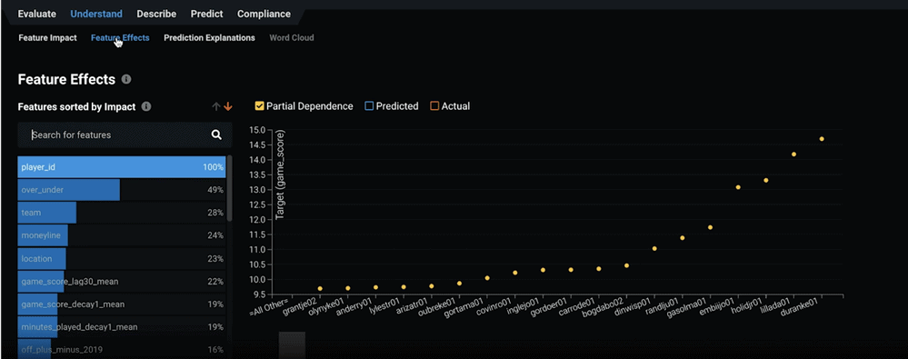
You can also examine how these features are affecting predictions using Feature Effects (shown in Figure 12), which is also in the Understand division. Below, you can see an example of how the number of in-patient visits increases the likelihood of readmission. This is calculated using a model-agnostic approach called partial dependence.

Feature Impact and Feature Effects show you the global impact of features on your predictions. You can find how features are impacting your predictions locally under Understand > Prediction Explanations (Figure 13).

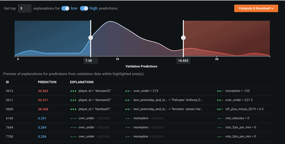
Here you will find a sample of row-by-row explanations that tell you the reason for the prediction, which is very useful for communicating modeling results to non-data scientists. Someone who has domain expertise should be able to look at these specific examples and understand what is happening. You can get these for every row within your dataset.

Model Deployment

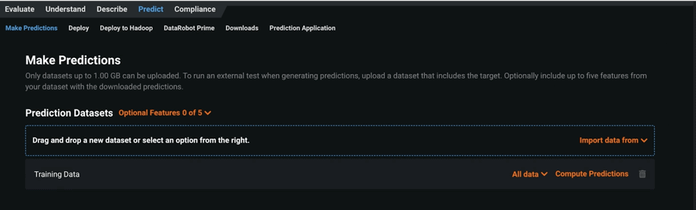
There are four ways to get data out of DataRobot under the Predict division

• The first is to use the GUI in the Make Predictions tab to simply upload scoring data and compute directly in DataRobot (Figure 14). You can then download the results with the push of a button. Customers usually use this for ad-hoc analysis or when they don’t have to make predictions very often.

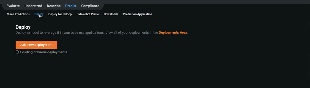
• You can create a REST API endpoint to score data directly from your applications in the Deploy tab (shown in Figure 15). An independent prediction server is available to support low latency, high throughput prediction requirements. You can set this up to score your data periodically.

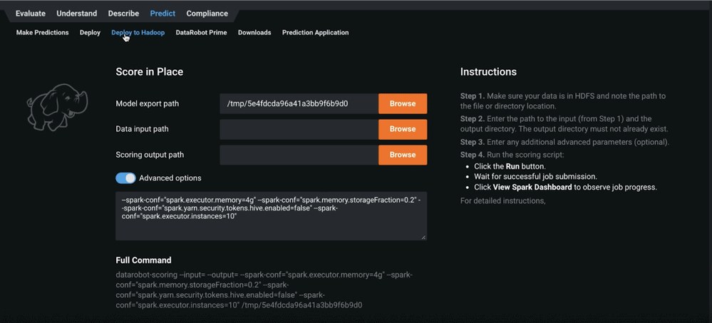
• Through the Deploy to Hadoop tab (Figure 16), you can deploy to Hadoop. Users who do this generally have large data and are using Hadoop.

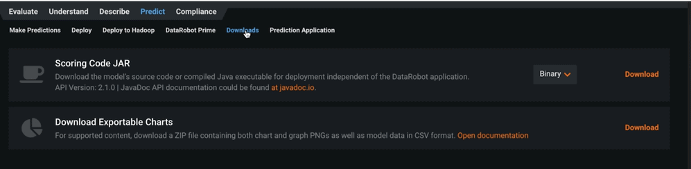
• Finally, using the Downloads tab, you can download the scoring code to score your data outside of DataRobot (shown in Figure 17). Customers who do this generally want to score their data off of a network or at a very low latency.