

Rock Solid AI: Using Geological Data for Oil and Gas Exploration
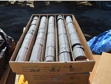
Core samples used to train machine learning model
Lithofacies are characteristics of rock such as chemical composition and permeability. Determining the facies of various rock formations in a reservoir is central to oil and gas development, as it helps characterize the reservoir and predict where recoverable oil or gas is likely to be. While core samples can be used to directly determine the facies types in a well, core samples are expensive to recover and are not always available.
Wireline log data can be more readily gathered as an alternative to core samples. If log data is compared to labeled core samples, a statistical model can be built that predicts facies types using the log data. This makes it possible to build a reservoir model with fewer core samples and is an example of supervised machine learning – using models built from labeled data to make predictions on unlabeled data.
There are a number of applications of supervised machine learning in the oil and gas industry beyond predicting lithofacies, but there’s a catch – machine learning is hard. It’s time-consuming. There are tons of types of machine learning models out there, each of which needs to be coded, tuned, and deployed, slowing down widespread adoption of machine learning techniques.
This got us wondering, how well would DataRobot’s automated machine learning platform do if we used it to select and tune a machine learning model to predict lithofacies from wireline log data? If DataRobot could do the facies classification work for us, how many other use cases are there where we could rapidly build and deploy machine learning models?
The Dataset
The Council Grove dataset we used to build the models contains data from nine different wells and a total of roughly 4,000 measurements from those nine wells. The observations from each well have been labeled ahead of time using core samples. To ensure our model will generalize to new wells, we trained our models on samples from seven of the wells and then checked the predictions of the different models on the remaining two wells that the models have not seen before, which we call the ‘holdout’ wells.
Out-of-the-Box Model Prototyping
Framing the Problem
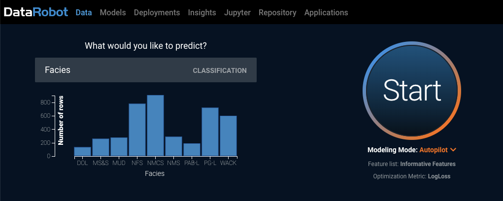
To get started, we can just drag and drop the dataset into DataRobot, and tell DataRobot to set samples from two of the wells aside as holdouts to test our models on at the end. Once we tell it to predict the ‘Facies’ columns, it recognizes this as a multiclass classification problem since we had nine different rock labels in our target.
Understanding the Best Performing Models
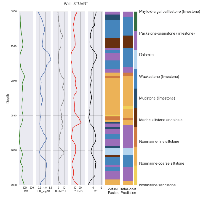
With no prior feature engineering, and by simply dragging and dropping the raw dataset into DataRobot, we were able to build a production-ready model that classified the facies types in the two holdout wells correctly on 65% percent of the samples. How? DataRobot built and compared 41 machine learning models including deep learning TensorFlow models, logistic regression models, and gradient-boosted, decision tree models. For each of these models, DataRobot provides complete transparency around preprocessing, feature engineering, and algorithmic parameters. By comparing the performance of different models on the two wells we set aside, DataRobot progressively narrowed down the models to one approach that best fit our sample data. Not bad for about half an hour of modeling work!
If we look at a cross-section from one of the holdout wells, we can see how DataRobot’s predictions compare to the actual labeled rock facies for a sample section:
No Black Boxes
DataRobot found that a Random Forest model did best at predicting the facies types on the holdout wells, but how? A black box model would be frustrating here. Without understanding how the random forest model arrived at its predictions, geologists and engineers wouldn’t be able to verify that the predictions make real-world sense and could be replicated in other datasets.
Fortunately, DataRobot’s models are transparent. We can examine each model blueprint, a documented diagram explaining each of the feature engineering and data preparation steps leading up to the final model. We can also check the Feature Impact charts, which tell us which attribute in the well log data is most important for making the prediction:
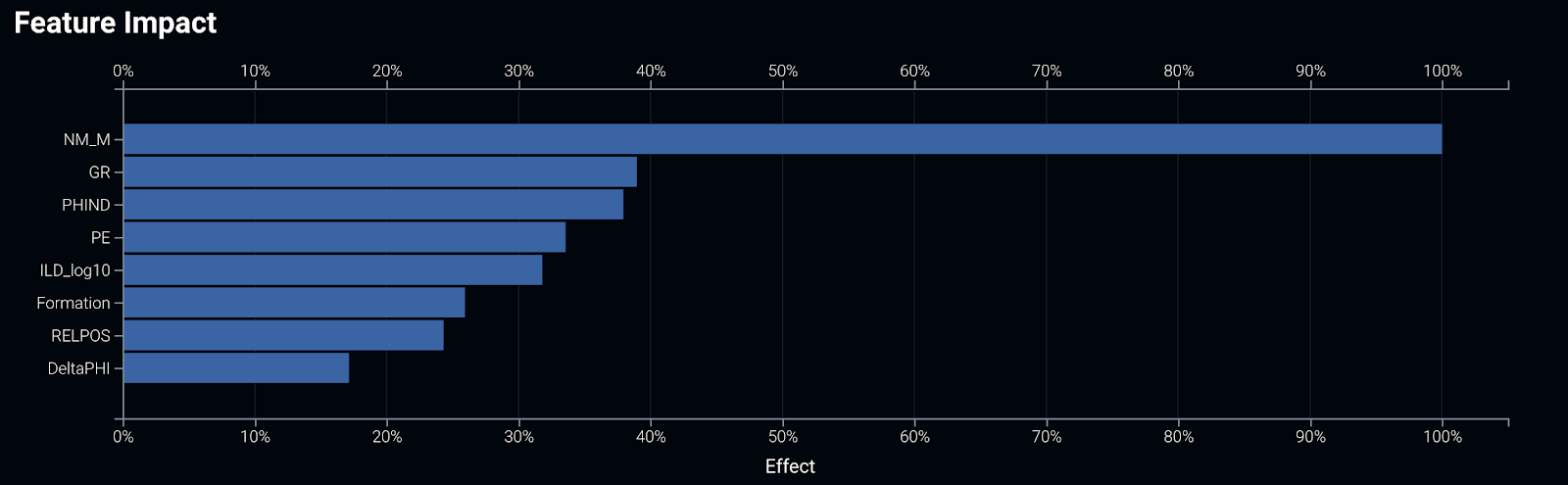
We can get a couple of takeaways from the feature impact chart. For one, the ‘Nonmarine-marine indicator’ column in our dataset is the feature that provides the most signal to distinguish facies types. But, just as important, we can see that the model is also picking up on significant signals from the other features we gave it to learn from.
The Confusion Matrix
Typically, when we build a model to distinguish multiple classes from one another, we want to drill down beyond the headline accuracy to understand where our model works well and where it is getting confused. This could inform future modeling iterations, or just help us to understand where we may need to gather more data to improve our ability to classify rock types.
Glancing at the whole 9-class confusion matrix, we can see the model does a pretty good job of identifying dolomite and limestone, but struggles with nonmarine sandstone:
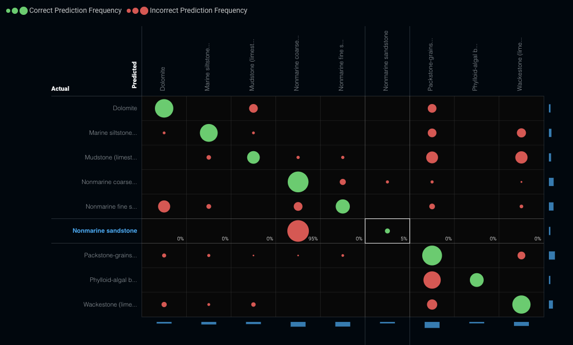
If we use DataRobot to drill down into the nonmarine sandstone predictions, we can begin to see a pattern. For 75% of the samples, what the model thought were nonmarine siltstone were, in fact, nonmarine coarse siltstone (presumably a rock type with similar characteristics).
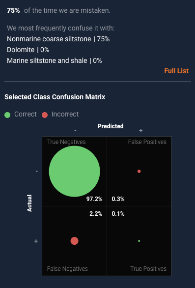
This type of analysis is where domain expertise becomes critical. How important is it to distinguish between the sandstone and siltstone samples as we build a reservoir model? If it is critical, we may need to explore different modeling techniques or figure out a way to gather data that would distinguish the two. If not, we may be satisfied with the model as is.
Typically, at this point, we could begin a few modeling iterations to get our model classification performance where we want it to be. For example, we know that facies at different depths aren’t random; certain facies tend to follow other facies. We could use data augmentation techniques to create new features that take account of known stacking patterns. Or we could use DataRobot’s modeling API to build a series of one-vs.-rest models to introduce some model diversity in our predictions, rather than relying on a single model to predict all rock facies. With DataRobot’s rapid modeling, we could try far more approaches than would be feasible otherwise.
Beyond Facies Classification
This exercise demonstrates how rapid and explainable automated modeling can open up the possibilities for applying machine learning in the oil and gas industry. If we can build a prototype model of a 9-class classification problem in minutes, the possibilities around predicting well output, favorable well location, or even maintenance and logistics are endless. Explainable models allow experts to understand how the model is picking up on signal and improve model performance, without the need to spend weeks fiddling with the machine learning aspect. Happy modeling!

About the Author
Dave Heinicke is a Customer-Facing Data Scientist at DataRobot focused on customer success with the platform. With a background in mechanical engineering focused on the energy industry prior to DataRobot, Dave works closely with customers in the oil and gas industry, manufacturing, logistics and more to ensure they derive value from their data.
-
How to Choose the Right LLM for Your Use Case
April 18, 2024· 7 min read -
Belong @ DataRobot: Celebrating 2024 Women’s History Month with DataRobot AI Legends
March 28, 2024· 6 min read -
Choosing the Right Vector Embedding Model for Your Generative AI Use Case
March 7, 2024· 8 min read
Latest posts
