This short tutorial will not only guide you through some basic data analysis methods but it will also show you how to implement some of the more sophisticated techniques available today. We will look into traffic accident data from the National Highway Traffic Safety Administration and try to predict fatal accidents using state-of-the-art statistical learning techniques. If you are interested, download the code at the bottom and follow along as we work through a real world data set. This post is in R while a companion post covers the same techniques in Python.

Getting started in R

The swirl package is designed to teach people R. You can visit their website to see links to YouTube videos on installing R on both Mac and Windows.

You can download R directly using these links for the Windows installer or the Mac package. The R install packages are hosted by the CRAN project. Just bear in mind that these are large files (60-70MB) and will take some time to download and install.

We suggest you install and view this file in RStudio. After you have installed R, download and run the installer for Rstudio. We recommend using RStudio as the IDE, but you can also use the R console directly if you choose.

If you open this file in RStudio, you can see the code is stored in “cells”“ or “chunks” like this:

# This is a code cell

You can also enter the code in the cells directly at the R command prompt.

If you click in a cell, you can run the code in that cell by selecting “Run Current Chunk” under the Chunks menu.

Try running the code in the following cell, which will load the libraries needed for the rest of this tutorial.

library("glmnet")  # For ridge regression fitting. It also supports elastic-net and LASSO models
## Loading required package: Matrix
## Loaded glmnet 1.9-5
library("gbm")  # For Gradient-Boosting
## Loading required package: survival
## Loading required package: splines
## Loading required package: lattice
## Loading required package: parallel
## Loaded gbm 2.1
library("rpart")  # For building decision trees

If you get an error, delete the # and run the following code chunk to install the needed packages.

# install.packages(c('glmnet', 'gbm', 'rpart'))

If you prefer, you can download a version with just the R code here, which you can load into R via the source command.

Now that you have R installed, we can start with our analysis. Inside RStudio, select “Run Next Chunk” under the “Chunks” menu to run the examples one at a time.

Get some data

Being able to play with data requires having the data available, so let’s take care of that right now. The National Highway Traffic Safety Administration (NHTSA) has some really cool data that they make public. The following code snippet will take care of downloading the data to a temporary file, and extract the file we are interested in, “PERSON.TXT”, from the zipfile. Finally, it loads the data into R. The zip is 14.9 MB so it might take some time to run – it is worth the wait! This is really cool data.

temp <- tempfile()
download.file("ftp://ftp.nhtsa.dot.gov/GES/GES12/GES12_Flatfile.zip", temp,
    quiet = TRUE)
accident_data_set <- read.delim(unz(temp, "PERSON.TXT"))
unlink(temp)

With our data downloaded and readily accessible, we can start to play around and see what we can learn from the data. Many of the columns have an encoding that you will need to read the manual in order to understand; it might be useful to download the PDF so you can easily refer to it. Again, we will be looking at PERSON.TXT, which contains information about individuals involved in road accidents.

print(sort(colnames(accident_data_set)))
##  [1] "AGE"        "AGE_IM"     "AIR_BAG"    "ALC_RES"    "ALC_STATUS"
##  [6] "ATST_TYP"   "BODY_TYP"   "CASENUM"    "DRINKING"   "DRUGRES1"
## [11] "DRUGRES2"   "DRUGRES3"   "DRUGS"      "DRUGTST1"   "DRUGTST2"
## [16] "DRUGTST3"   "DSTATUS"    "EJECT_IM"   "EJECTION"   "EMER_USE"
## [21] "FIRE_EXP"   "HARM_EV"    "HOSPITAL"   "HOUR"       "IMPACT1"
## [26] "INJ_SEV"    "INJSEV_IM"  "LOCATION"   "MAKE"       "MAN_COLL"
## [31] "MINUTE"     "MOD_YEAR"   "MONTH"      "PERALCH_IM" "PER_NO"
## [36] "PER_TYP"    "PJ"         "P_SF1"      "P_SF2"      "P_SF3"
## [41] "PSU"        "PSUSTRAT"   "REGION"     "REST_MIS"   "REST_USE"
## [46] "ROLLOVER"   "SCH_BUS"    "SEAT_IM"    "SEAT_POS"   "SEX"
## [51] "SEX_IM"     "SPEC_USE"   "STRATUM"    "STR_VEH"    "TOW_VEH"
## [56] "VE_FORMS"   "VEH_NO"     "WEIGHT"

Clean up the data

One prediction task you might find interesting is predicting whether or not a crash was fatal. The column INJSEV_IM contains imputed values for the severity of the injury, but there is one value that might complicate analysis – level 6 indicates that the person died prior to the crash.

table(accident_data_set$INJSEV_IM)
##
##      0      1      2      3      4      5      6
## 100840  19380  20758   9738   1178   1179      4

Forntunately, there are only four of those cases within the dataset, so it is not unreasonable to ignore them during our analysis. However, we will find that a few of these columns have missing values:

accident_data_set <- accident_data_set[accident_data_set$INJSEV_IM != 6, ]
for (i in 1:ncol(accident_data_set)) {
  if (sum(as.numeric(is.na(accident_data_set[, i]))) > 0) {
    num_missing <- sum(as.numeric(is.na(accident_data_set[, i])))
    print(paste0(colnames(accident_data_set)[i], ": ", num_missing))
  }
}
## [1] "MAKE:  5162"
## [1] "BODY_TYP:  5162"
## [1] "MOD_YEAR:  5162"
## [1] "TOW_VEH:  5162"
## [1] "SPEC_USE:  5162"
## [1] "EMER_USE:  5162"
## [1] "ROLLOVER:  5162"
## [1] "IMPACT1:  5162"
## [1] "FIRE_EXP:  5162"

For this analysis, we will just drop these rows (they are all the same rows) – but you certainly don’t have to do that. In fact, maybe there is a systematic data entry error that is causing them to be interpreted incorrectly. Regardless of the way you cleanup this data, we will most assuredly want to drop the column INJ_SEV, as it is the non-imputed version of INJSEV_IM and is a pretty severe data leak – there are others as well.

rows_to_drop <- which(apply(accident_data_set, 1, FUN = function(X) {
    return(sum(is.na(X)) > 0)
}))
data <- accident_data_set[-rows_to_drop, ]
data$INJ_SEV <- NULL

One more preprocessing step we’ll do is to transform the response. If you flip to the manual it shows that category 4 is a fatal injury – so we will encode our target as such.

data$INJSEV_IM <- as.numeric(data$INJSEV_IM == 4)
target <- data$INJSEV_IM

Now, we model!

We have predictors, we have a target, now it is time to build a model. We will be using ordinary least squares, Ridge Regression and Lasso Regression, both forms of regularized Linear Regression, a Gradient Boosting Machine (GBM), and a CART decision tree, to have some variety in modeling methods. These are just some representatives from the many packages available in R, which gives you access to quite a few machine learning techniques.

Don’t be alarmed if this cell block takes quite a bit of time to run – the data is of non-negligible size. Additionally the ridge classifier is running several times to compute an optimal penalty parameter, and the gradient boosting classifier is building many trees in order to produce its ensembled decisions. There is a lot of computation going on under the hood, so get up and take a break if you need.

# Split the data into test and train sets
train_rows <- sample(nrow(data), round(nrow(data) * 0.5))
traindf <- data[train_rows, ]
testdf <- data[-train_rows, ]

First the linear model:

OLS_model <- lm(INJSEV_IM ~ ., data = traindf)

Then the GBM:

print("Started Training GBM")
## [1] "Started Training GBM"
# GBM is easier to process as a data matrix
response_column <- which(colnames(traindf) == "INJSEV_IM")
trainy <- traindf$INJSEV_IM
gbm_formula <- as.formula(paste0("INJSEV_IM ~ ", paste(colnames(traindf[, -response_column]),
collapse = " + ")))
gbm_model <- gbm(gbm_formula, traindf, distribution = "bernoulli", n.trees = 500,
bag.fraction = 0.75, cv.folds = 5, interaction.depth = 3)
## Warning: variable 16: STR_VEH has no variation.
## Warning: variable 47: DRUGTST2 has no variation.
## Warning: variable 48: DRUGTST3 has no variation.
## Warning: variable 50: DRUGRES2 has no variation.
## Warning: variable 51: DRUGRES3 has no variation.
## Warning: variable 56: LOCATION has no variation.
print("Finished Training GBM")
## [1] "Finished Training GBM"
# For glmnet we make a copy of our dataframe into a matrix
trainx_dm <- data.matrix(traindf[, -response_column])
print("Started fitting LASSO")
## [1] "Started fitting LASSO"
lasso_model <- cv.glmnet(x = trainx_dm, y = traindf$INJSEV_IM, alpha = 1)
print("Finished fitting LASSO")
## [1] "Finished fitting LASSO"
print("Started fitting RIDGE")
## [1] "Started fitting RIDGE"
ridge_model <- cv.glmnet(x = trainx_dm, y = traindf$INJSEV_IM, alpha = 0)
print("Finished fitting RIDGE")
## [1] "Finished fitting RIDGE"

And finally, we make a decison tree:

dtree_model <- rpart(INJSEV_IM ~ ., traindf)

Now we can make predictions. For the GBM, we need to decide on how many trees to predict with. The following will plot how well the GBM performs at each of the 500 iterations, one for each additional tree. We want to minimize the green line, which represents the model performance on test data.

gbm_perf <- gbm.perf(gbm_model, method = "cv")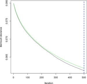

Notice that since the curve is still decreasing, we could try training more trees at the expense of more computation.

Now we can make predictions using our trained models:

predictions_ols <- predict(OLS_model, testdf[, -response_column])
## Warning: prediction from a rank-deficient fit may be misleading
predictions_gbm <- predict(gbm_model, newdata = testdf[, -response_column],
    n.trees = gbm_perf, type = "response")
testx_dm <- data.matrix(testdf[, -response_column])
predictions_lasso <- predict(lasso_model, newx = testx_dm, type = "response",
s = "lambda.min")[, 1]
predictions_ridge <- predict(ridge_model, newx = testx_dm, type = "response",
s = "lambda.min")[, 1]
predictions_dtree <- predict(dtree_model, testdf[, -response_column])

We can now assess model performance on the test set. We will be using the metric of area under the ROC curve. A perfect classifier would score 1.0 while purely random guessing would score 0.5.

print("OLS: Area under the ROC curve:")
## [1] "OLS: Area under the ROC curve:"
auc(testdf$INJSEV_IM, predictions_ols)
## [1] 0.9338
print("Rdige: Area under the ROC curve:")
## [1] "Rdige: Area under the ROC curve:"
auc(testdf$INJSEV_IM, predictions_ridge)
## [1] 0.9348
print("LASSO: Area under the ROC curve:")
## [1] "LASSO: Area under the ROC curve:"
auc(testdf$INJSEV_IM, predictions_lasso)
## [1] 0.9339
print("GBM: Area under the ROC curve:")
## [1] "GBM: Area under the ROC curve:"
auc(testdf$INJSEV_IM, predictions_gbm)
## [1] 0.921
print("Decision Tree: Area under the ROC curve:")
## [1] "Decision Tree: Area under the ROC curve:"
auc(testdf$INJSEV_IM, predictions_dtree)
## [1] 0.8473

What else can I do?

We have a blogpost that goes into more detail about regularized linear regression, if that is what you are interested in. It would also be good to look at the various other packages in R, listed on CRAN under the task “MachineLearning” available here. Beyond that, here are a few challenges that you can undertake to help you hone your data science skills.

Data Prep

If it wasn’t obvious in the blog post, the column STRATUM is a data leak (it encodes the severity of the crash). Which other columns contain data leaks? Can you come up with a rigorous method to generate candidates for deletion without having to read the entire GES manual?

And while we are considering data preparation, consider the column REGION. Any regression model will consider the West region to be 4 times more REGION-y than the Northeast – that just doesn’t make sense. Which columns could benefit from being encoded as factor levels, rather than as numeric? To change a column into a factor, use the as.factor command.

Which is the best model?

How good of a model can you build for predicting fatalities from car crashes? First you will need to settle on a metric of “good” – and be prepared to reason why it is a good metric. How bad is it to be wrong? How good is it to be right?

In order to avoid overfitting you will want to separate some of the data and hold it in reserve for when you evaluate your models – some of these models are expressive enough to memorize all the data!

Which is the best story?

Of course, data science is more than just gathering data and building models – it’s about telling a story backed up by the data. Do crashes with alcohol involved tend to lead to more serious injuries? When it is late at night, are there more convertibles involved in crashes than other types of vehicles (this one involves looking at a different dataset with the GES data)? Which is the safest seat in a car? And how sure can you be that your findings are statistically relevant?

Good luck coming up with a great story!

Download Notebook Download R File

This post was written by Mark Steadman and Dallin Akagi.