


Best Practice of Using Data Science Competitions Skills to Improve Business Value
Rapid advances in machine learning in recent years have begun to lower the technical hurdles to implementing AI, and various companies have begun to actively use machine learning. Companies are emphasizing the accuracy of machine learning models while at the same time focusing on cost reduction, both of which are important. Of course, finding a compromise is necessary to a certain degree, but rather than simply compromising, finding the optimal solution within that trade-off is the key to creating maximum business value.
This article presents a case study of how DataRobot was able to achieve high accuracy and low cost by actually using techniques learned through Data Science Competitions in the process of solving a DataRobot customer’s problem.
The Best Way to Achieve Both Accuracy and Cost Control
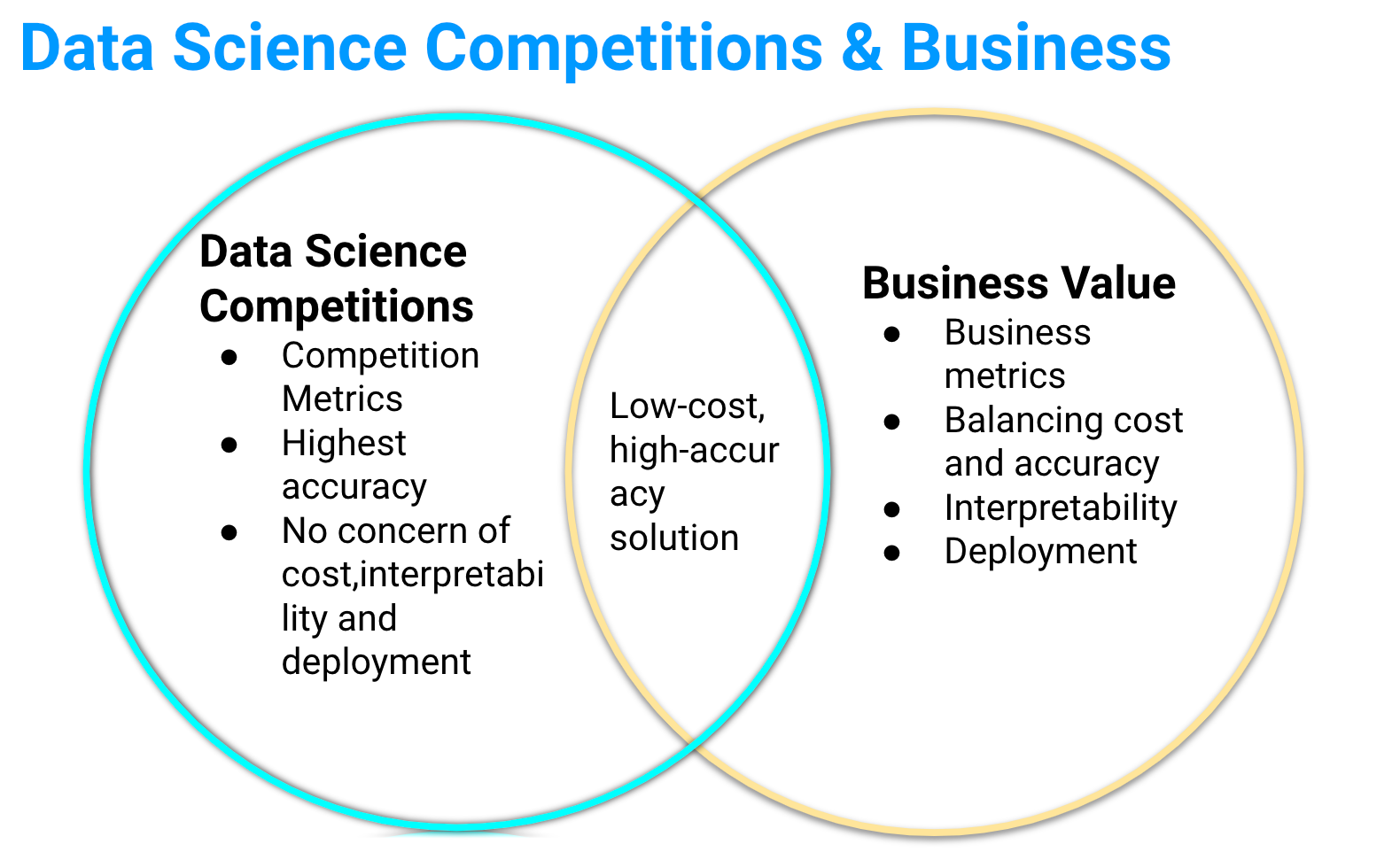
As a DataRobot data scientist, I have worked with team members on a variety of projects to improve the business value of our customers. In addition to the accuracy of the models we built, we had to consider business metrics, cost, interpretability, and suitability for ongoing operations. Ultimately, the evaluation is based on whether or not the model delivers success to the customers’ business.
On the other hand, in the Data Science Competitions, which I have participated in for many years as a hobby, the data and evaluation criteria are basically prepared from the beginning, so basically all you have to do is focus on improving accuracy. While the application of cutting-edge technology and the ability to come up with novel ideas are often the deciding factors, a simple solution based on an understanding of the essence of the problem can often be the winning solution.
While there are many differences between Data Science Competitions and business, there are also similarities. That commonality is that low-cost, high-accuracy solution methods, or approaches of excellence, can have a significant impact on results. In this blog post, we would like to present some examples of actual cases in which noise reduction had a significant effect in real-world applications, and in which powerful features were obtained. Finding such good solutions is not only useful to win at Data Science Competitions, but also to maximize business value.
Sensor Data Analysis Examples
The accuracy of machine learning models is highly dependent on the quality of the training data. Without high-quality data, no matter how advanced the model is, it will not produce good results. Real data is almost always a mixture of signal and noise, and if you include that noise in the model, it will be difficult to capture the signal.
Especially in time series data analysis, there are many situations in which there are severe fluctuations and consequent noise. For example, data measured by sensors can contain all kinds of noise due to sensor malfunctions, environmental changes, etc., which can lead to large prediction errors. Another example is website access data, where the presence of spamming, search engine crawlers, etc. can make it difficult to analyze the actions of ordinary users. Distinguishing between signal and noise is one important aspect of machine learning model improvement. To improve model accuracy, it is necessary to increase the signal-to-noise ratio (SNR), and it is common practice to try to extract more signals by spending a lot of time and effort on feature engineering and modeling, but this is often not a straightforward process. When comparing the two approaches, signal enhancement and noise reduction, noise reduction is easier and more effective in many cases.
The following is a case where I have succeeded in significantly improving accuracy by using a noise reduction method in practice. The customer’s challenge was to detect predictive signs in the manufacturing process of a certain material. If the various observed values measured by sensors in the equipment could be predicted, it would be possible to control manufacturing parameters and reduce fuel costs. The bottleneck here was the very low quality of the data, which was very noisy, including periods of stable operation and periods of shutdown. Initially, the customer tried modeling using statistical methods to create typical features, such as moving averages, but the model metrics (R-square) was only 0.5 or less. The larger the value, the better the model represents the data, and the smaller the value, the less well it represents the data. Therefore, a value below 0.5 could not be said to be highly accurate, and in fact the model was not practical. Moving average features can reduce noise to a certain degree, but the noise was so large that it was insufficient.
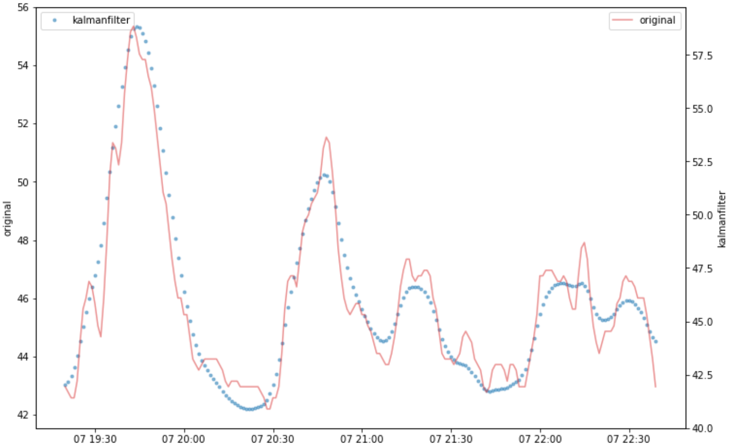
At that time, I thought of a solution from the top team in a Data Science Competitions called Web Traffic Time Series Forecasting. The competition was to predict Wikipedia’s pageview, but it was an analysis problem for very noisy time series data. The winning team was able to use RNN seq2seq to learn to robustly encode and decode even noisy data, which was a great solution. More interesting was the 8th place team’s solution, which used a kalman filter rather than a machine learning model to remove noise, and then added statistical methods to build a robust prediction model, which was extremely simple and powerful. I remember being impressed at the time that this was a highly productive technology that should be pursued in practice.
The Kalman filter is a method for efficiently estimating the invisible internal “state” in a mathematical model called a state-space model. In the state-space model, for example, information obtained from sensors is used as “observed values” from which the “state” is estimated, and control is performed based on this. Even if there is noise in the “observed values,” the “state” will eliminate the noise and become the original correct observed values.
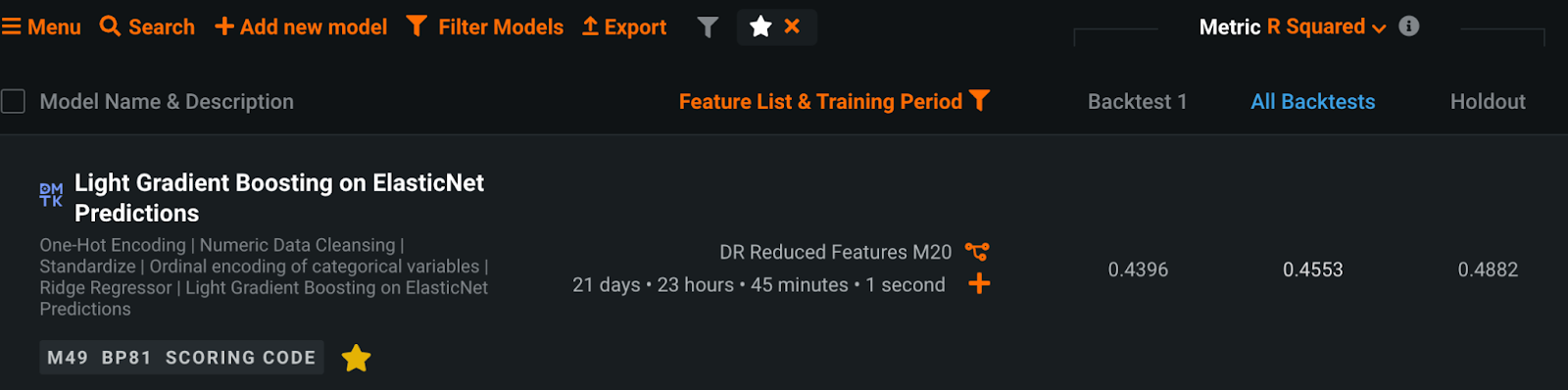
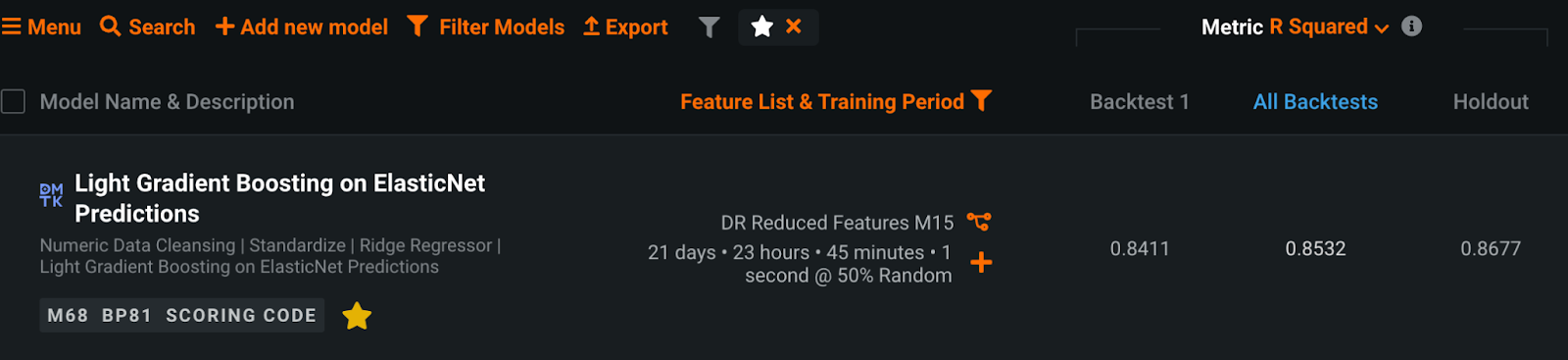
After processing all the observed values using the Kalman filter, I created moving average features and trained a model using DataRobot. The R-square, which was less than 0.5 using the conventional method, improved to more than 0.85 at once, a significant improvement that was like magic. Moreover, the process took only a few dozen seconds for several tens of thousands of rows of data, and a highly accurate forecasting model was realized at a low cost.
There is a library called pykalman that can handle Kalman filters in Python, which is simple to use and useful.
from pykalman import KalmanFilter

def Kalman1D(observations,damping=1):
    observation_covariance = damping
    initial_value_guess = observations[0]
    transition_matrix = 1
    transition_covariance = 0.1
    initial_value_guess

    kf = KalmanFilter(
            initial_state_mean=initial_value_guess,
            initial_state_covariance=observation_covariance,
            observation_covariance=observation_covariance,
            transition_covariance=transition_covariance,
            transition_matrices=transition_matrix
        )

    pred_state, state_cov = kf.smooth(observations)
    return pred_state

observation_covariance = 1 # <- Hyperparameter Tuning
df['sensor_kf'] = Kalman1D(df['sensor'].values, observation_covariance)
Examples of Voice Data Analysis
The accuracy of machine learning models is limited only by the quality of the training data, but if you can master the techniques of feature engineering, you can maximize their potential. Feature creation is the most time-consuming part of the machine learning model building process, and it is not uncommon to spend an enormous amount of time experimenting with different feature combinations. However, if we can understand the essence of the data and extract features that can represent business knowledge, we can build highly accurate models even with a small number of features.
I would like to introduce one of the cases where I have improved accuracy with simple features in practice. The customer’s problem was a process to control engine knocking in automobiles. Conventionally, the level of engine knocking was determined by the hearing of a skilled person, but this required special training, was difficult to determine, and resulted in variation. If this knock leveling could be automated, it would result in significant cost savings. The first baseline model we created used spectrograms of speech waveform data, statistical features, and spectrogram images. This approach got us to an R-squared of 0.7, but it was difficult to improve beyond that.
I thought of the solutions of the top team in a Data Science Competition for LANL Earthquake Prediction. The competition was to predict the time-to-failure of an earthquake using only acoustic data obtained from experimental equipment used in earthquake research. The winning team and many other top teams used an approach that reduced overfitting and built robust models by reducing the number of features to a very small number, including the Mel Frequency Cepstrum (MFCC).
MFCC is thought to better represent the characteristics of sounds heard by humans by stretching the frequency components that are important to human hearing and increasing their proportion in the overall cepstrum. In addition, by passing through an Nth-order Melfilter bank, the dimension of the cepstrum can be reduced to N while preserving the features that are important to human hearing, which has the advantage of reducing the computational load in machine learning.
For the task of determining the level of engine knocking, this MFCC feature was very well suited, and by adding it to this customer’s model, we were able to significantly improve the R-square to over 0.8. Again, high accuracy was achieved at a low cost, and processing could be completed in tens of seconds for several hundred audio files.
There is a library called librosa that can extract MFCC features in Python, and sample code is provided below for your reference.
import librosa

fn = 'audio file path'
y, sr = librosa.core.load(fn)
mfcc = librosa.feature.mfcc(y=y, sr=sr, n_mfcc=20)
mfcc_mean = mfcc.mean(axis=1)
Custom Model in DataRobot
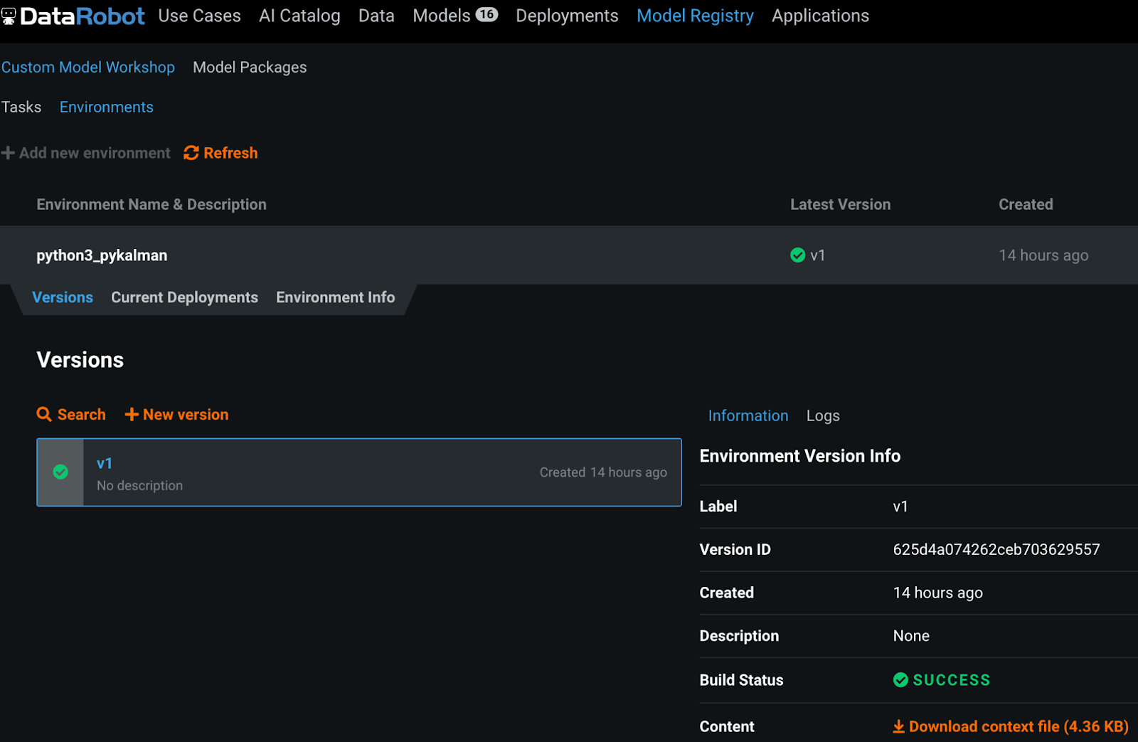
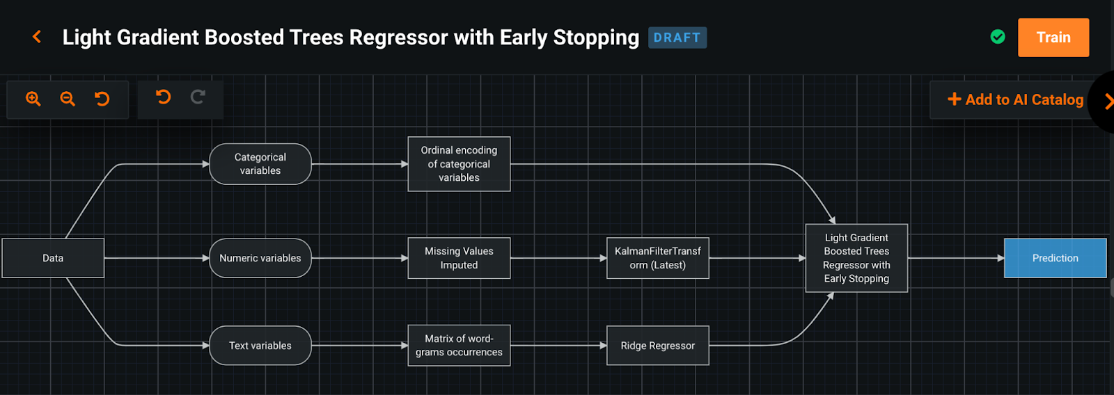
Now it is actually possible to use pykalman, librosa, etc. on the DataRobot platform. By combining the various built-in tasks in DataRobot with custom tasks designed by users in Python or R, users can easily build their own machine learning pipelines. In addition, custom container environments for tasks allow you to add dependencies at any time.
Summary
As we have explained, the key to both improving the accuracy and reducing the cost of machine learning models is not simply to compromise, but to find the optimal solution, based on a real customer case study of DataRobot, applying the concise yet powerful techniques learned from the Data Science Competitions. DataRobot Composable ML allows you to build custom environments, code tasks in Python or R, and work with the DataRobot platform to build optimal models. We also hope you will take advantage of Composable ML, a new feature that combines high productivity with full automation and customizability.

Senkin Zhan is a Senior Execution Data Scientist at DataRobot. Senkin develops end-to-end enterprise AI solutions with DataRobot AI Platform for customers across industry verticals. He is also a Kaggle competition grandmaster who won many gold medals.
-
How to Choose the Right LLM for Your Use Case
April 18, 2024· 7 min read -
Belong @ DataRobot: Celebrating 2024 Women’s History Month with DataRobot AI Legends
March 28, 2024· 6 min read -
Choosing the Right Vector Embedding Model for Your Generative AI Use Case
March 7, 2024· 8 min read
Latest posts
